Rev. IBRACON Estrut. Mater. vol.8 número1

(1)

Thermal analysis of two-dimensional structures in ire

Análise térmica de estruturas bidimensionais em

situação de incêndio

a_{Escola Politécnica da Universidade de São Paulo.} b_{Universidade Federal de Santa Catarina.}

Received: 12 Aug 2014 • Accepted: 17 Nov 2014 • Available Online: 03 Feb 2014

Abstract

Resumo

The structural materials, as reinforced concrete, steel, wood and aluminum, when heated have their mechanical proprieties degraded. In ire, the

structures are subject to elevated temperatures and consequently the load capacity of the structural elements is reduced. The Brazilian and

Eu-ropean standards show the minimal dimensions for the structural elements had an adequate bearing capacity in ire. However, several structural

checks are not contemplated in methods provided by the standards. In these situations, the knowledge of the temperature distributions inside of structural elements as function of time of exposition is required. The aim of this paper is present software developed by the authors called ATERM. The software performs the thermal transient analysis of two-dimensional structures. The structure may be formed of any material and heating is provided by means of a curve of temperature versus time. The data input and the visualization of the results is performed thought the GiD soft-ware. Several examples are compared with software Super TempCalc and ANSYS. Some conclusions and recommendations about the thermal analysis are presented.

Keywords: ire, thermal analysis, inite element method, software.

Os materiais utilizados na construção civil, tais como o concreto armado, aço, madeira e alumínio, sofrem degradação de suas propriedades me-cânicas quando aquecidos. Em situação de incêndio, as estruturas são submetidas a elevadas temperaturas e, consequentemente, os elementos estruturais perdem sua capacidade portante. As normas brasileira e europeia apresentam algumas dimensões mínimas para os elementos

estru-turais apresentarem capacidade resistente adequada em situação de incêndio. Porém, diversas veriicações estruestru-turais não são contempladas

nos métodos apresentados pelas normas. Nessas situações, é necessário o conhecimento da distribuição de temperaturas no interior do elemen-to estrutural em função do tempo de exposição ao incêndio. O objetivo deste artigo é apresentar um programa de computador desenvolvido pelos autores denominado de ATERM. O programa efetua a análise térmica de estruturas bidimensionais em regime transiente por meio do método dos

elementos initos. A estrutura pode ser constituída de qualquer material e o aquecimento é fornecido por meio de uma curva de temperaturas em

função do tempo. A entrada de dados e visualização dos resultados é realizada por meio do programa GiD. Diversos resultados foram

compara-dos ao programa Super Tempcalc e ao programa ANSYS. Ao inal do artigo são extraídas algumas conclusões e recomendações sobre a análise

térmica de estruturas em situação de incêndio.

Palavras-chave: incêndio, análise térmica, método dos elementos initos, software.

I. PIERIN a

igorpierin@usp.br

V. P. SILVA a

valpigss@usp.br

H. L. LA ROVERE b

(2)

1. Introduction

In several engineering areas, it is very important to know the tem-perature distribution within a solid body. In civil engineering,

es-pecially in the structures ire design and in the design of roll com -pacted concrete dams, the interest in the study of temperature

ield evolution within structural elements have signiicantly grown

in recent years.

Concrete structure ire design is ruled by ABNT NBR 15200:2012 [1]. This standard presents simpliied methods and allows using advanced methods for checking structural elements in ire, besides the use of tests. The simpliied methods are applicable in several

situations. Nonetheless, there are design situations that cannot be

represented by them, asking for a more reined analysis. The use of advanced methods for verifying the ire safety of struc -tures requires models for determining the development and distri-bution of temperatures in structural parts.

The thermal analysis may be based on the heat transfer principles and hypotheses. The model adopted may take into consideration the relevant thermal actions and the variation in thermal proper-ties. When relevant, the effects of non-uniform thermal exposition and heat transfer through components of adjacent constructions should be included.

This paper presents a formulation for the thermal analysis of

two-dimensional structures using inite elements. This formulation was

implemented in a piece of software named ATERM [2], developed by the authors using FORTRAN 90 language. For data input and

visualization of the ield of temperatures, GiD [3] software is used.

For the validation of results, comparisons were made using Super Tempcalc (STC) [4], developed in Lund, Sweden. STC began be-ing developed in 1985 for the thermal analysis of two-dimensional structures. The software was checked against several

experimen-tal tests since its irst version and was used for elaborating Euro -code 2 part 1.2 [5].

The results obtained by means of the ATERM [2] software will also be compared to that obtained by ANSYS [6]. SOLID70 elements will be used in the models for the thermal analysis. Convection and radiation effects will be simulated by means of the SURF152 element using one extra node. Models constructed in ANSYS software are tridimensional, but they can be compared to the two-dimensional models obtained by ATERM because there is no temperature variation along the longitudinal axis of the structural element.

ATERM was also used by SILVA [7] in the study of reinforced

con-crete columns in ire. In that study, a collection of isotherms for

several cross sections was created.

2. Finite elements method

In its beginning, the Finite Elements Method was applied to me-chanics problems in structural engineering. The thermal analysis

was the irst non-structural area to use it for modelling engineer

-ing problems. The determination of the ield of temperatures within the structural element is the irst step for structure ire analysis.

Temperature distribution affects the stress distribution within the structural element.

Heat propagates within concrete by conduction. This phenomenon

is governed by Poisson’s equation, which, in its two-dimensional form, is given by equation (1).

(1)

Q

c

x

y

t

q

l

æ

l

ö

r

¶

æ

¶

_{ö +}

¶

_{+ =}

¶

ç

÷

ç

÷

¶

è

¶

ø

¶

è

¶

ø

&

¶

In equation (1),

λ

is the material thermal conductivity,

Q



is the internally generated heat per volume unit per time,

ρ

is the den-sity, c is the speciic heat, θ is the temperature and t is the time. To solve equation (1), it is necessary to impose the boundary and initial conditions of the mathematical model. The general bound-ary conditions of a structure subjected to Poisson’s equation are the Dirichlet and Neumann’s conditions. Dirichlet’s condition, or prescribed temperature, supposes that, for any instant, the

tem-perature in one part of the boundary is known. In ire analysis of

structures, Dirichlet’s condition is not important, for it does not take into consideration the heat transfer by convection and radiation.

Neumann’s condition supposes that the heat low in one part of the

boundary,

q



, is, for any instant, known. Mathematically, this condi-tion can be written by equacondi-tion (2), that is, the derivative of the

tem-perature ield in relation to the normal to the boundary surface, n.

(2)

q

n

q

l

¶

-

=

¶

&

One adiabatic, or thermally insulated, surface can be simulated by

imposing zero heat low (

q



=

0

).

The convection and radiation phenomena are included into the nu-merical model by means of Neumann’s boundary condition, which can be written by equation (3).

(3)

(

)

(

4 4

)

c

q

&

=

a q q

-

_¥

+

es

T

-

T

_¥

In equation (3),

α

_cis the convection coeficient,

θ

and

θ

_∞ are, respectively, the temperatures in the structure and out of it,

ε

is the emissivity,

σ

is the Stefan-Boltzmann constant,

T

and

T

_∞ are, respectively, the absolute temperatures in the structure and out of it.

By making the part due to radiation linear, equation (3) can be rewritten by means of equation (4),

(4)

(

)

(

)

(

)

c r

q

&

=

a q q

-

_¥

+

a q q

-

_¥

=

a q q

-

_¥

In equation (4),

α

_r is the coeficient for heat transfer by radiation provided by equation (5).

(5)

(

)(

2 2

)

r

T T

T

(3)

As the coeficient for heat transfer by radiation depends on the

structure temperature, the process becomes iterative.

The solution for the differential equation (1) can be numerically

ob-tained by the inite elements method (FEM). For the use of FEM,

it is necessary to write the weak problem formulation, which is ob-tained by equation (6).

(6)

0 w

Q c

d

x

y

t

q

l

r

W

é

¶

æ

¶

_{ö +}

¶

æ

¶

ö

_{+ -}

¶

ù

_{W =}

ê

_¶

ç

_è

_¶

÷

_ø

_¶

ç

_¶

÷

_¶

ú

è

ø

ë

û

ò

&

In equation (6), w is an arbitrary function named weight function and

Ω

is the problem dominium.

Integrating the two irst terms of equation (6) by parts and applying

Gauss’ Theorem, we obtain equation (7).

(7)

w

d

x

y

q

l

W

é

¶

æ

¶

_{ö +}

¶

æ

¶

ö

ù

_{W =}

ê

_¶

ç

_è

_¶

÷

_ø

_¶

ç

_¶

÷

ú

è

ø

ë

û

ò

S

w

x

l w

y

m dS

q

l

æ

¶

ö

=

_ç

+

_÷

-¶

¶

è

ø

ò

w

_d

x

y

q

l

W

æ

¶

ö

-

_ç

+

_÷

W

¶

è

ø

ò

In equation (7), S represents the problem boundary region and l

and m are the director cosines.

Substituting equation (7) in (6), we have equation (8).

(8)

0

S

wQd

w c d

w

l w

m dS

t

x

y

w

_d

x x y y

q

r

l

q

l

W W W

æ

ö

¶

W -

W+

_ç

+

_÷

-¶

_è

¶

_ø

æ

¶

¶ ¶ ¶

ö

-

_ç

+

_÷

W =

¶

¶ ¶ ¶

è

ø

ò

&

Discretizing the problem dominium in a inite number of elements

and using Galerkin Method, the set of interpolation functions N, as

weight functions, the temperature in any point of the inite element

can be approximated by equation (9).

(9)

(

, ,

)

n _ii i

x y t

N

q

=

å

q

In equation (9), n is the number of nodes of the element,

( )

,

i i

N

=

N x y

are the interpolation functions and

θ

_i are the nodal temperatures of the element.

Substituting equation (9) in (8), we get to the equations system (10), which represents the thermal balance in each fi-nite element.

(10)

0

e e e i i

i i e

A

i e i e

S S

N

_{N Q N c}

_dA

x x

y y

t

N

ldS

N

mdS

x

y

q

l

r

q

l

é

¶

ù

-

_ê

+

-

+

_ú

¶ ¶

¶

ë

û

¶

+

=

¶

ò

&

for i= 1 to n,

In equations (10), A and S represent the area and the surface of the element dominium.

The derivative of the temperature field in relation to the normal to the boundary surface, n, can be written in function of the director cosines, l and m, by means of equation (11).

(11)

l

m

n

x

y

q

¶

₌

¶

₊

¶

Substituting equations (2), (4) and (11) in equation (10), we obtain expression (12),

(12)

e i i e A

N

_dA

x x

y y

q

l

é

¶

ù

-

_ê

+

_ú

-¶ -¶

¶ ¶

ë

û

ò

(

)

0

e i e

S

N

a q q

¥

dS

-

ò

-

=

e i e e i e

A

N QdA

A

N c

t

dA

q

r

¶

-

-¶

ò

&

ò

Deining the interpolation function vector N and the nodal tempera-tures vector

θ

by means of expressions (13).

(13)

[

]

[

]

1 2 1

...

n n

T

n n

N N

N

q q

q

-=

=

N

q

Where n is the number of nodes of the element and N_iare the

interpolation functions of the inite element.

Thus, we can rewrite equation (9) in the matrix form by means of equation (14).

(14)

(

)

1

, ,

n _ii

i

x y t

N

q

=

å

=

N

q

We also deine the conductivity matrix of the material, for the case

(4)

(15)

0

0 l

l

é

ù

= ê

ú

ë

û

l

(16)

x

y

¶

ì ü

ï ï

_¶

ï ï

= í ý

_¶

ï ï

¶

ï ï

î þ

Ñ

Inserting equations (13) and (16) in equation (12) and rearranging the terms, we obtain the following set of equations (17).

(17)

( )

e e

e e e

T T

e e

A A

T T T

e e e

S A S

c

dA

t

dS

Q dA

dS

r

a

aq

_¥

¶

+

¶

=

+

ò

&

ò

N

N N

N

q

l

q

Ñ

The set of equations (17) can be rewritten in the matrix form by means of equation (18).

(18)

+

=

&

C

q

K

q

F

In equation (18),

θ



is the irst derivative of the temperatures ield in relation to time.

The total capacitance matrix (

K

) of the element is given by equa-tion (19).

(19)

_

cond conv rad

=

+

K K

K

The element conductivity matrix is given by equation (20).

(20)

e T cond

=

ò

_A

dA

e

K

B B

l

where

(21)

=

B

Ñ

N

And the matrix due to the combined effects of convection and ra-diation of the element is given by equation (22).

(22)

(

)

_

e

T

conv rad

=

ò

_S

a

c

+

a

r

dS

e

K

N N

q

We deine the thermal capacity of the material as the product den -sity (

ρ

) x speciic heat (

c

). Thus, the thermal capacity matrix (

C

) of the element is given by equation (23).

(23)

e

T

e A

r

c dA

=

ò

C

N

The vector of the consistent thermal actions (

F

) is given by ex-pression (24).

(24)

(

)

e e

T T

e c r e

A

Q dA

S

a

a q

¥

dS

=

ò

&

+

ò

+

F

N

In equation (24),

θ

∞is the temperature outside the structure.

Matrixes

N

and

B

depend on the type of element used in struc-ture discretizing.

In ATERM, we employ rectangular and triangular planes of four and three nodes, respectively, and two nodes special bar elements for considering convection and radiation heat transfer effects, which can be superimposed in any face of the plane elements. These

ele-ments are briely described in the following items. Further details on the used inite elements and the computational implementation

can be found in Pierin [2].

2.1 Four nodes rectangular element

The four-node plane rectangular inite element with sides 2a by 2b

used herein is represented in Figure 1.

The interpolation functions

N

_i are deined by means of equation (25).

(25)

1 1

1

4

i i i

x

y

N

x

y

æ

öæ

ö

=

_ç

+

_÷ç

+

_÷

è

øè

ø

to

i

=

1,2,3,4

By substituting equations (15), (21) and (25) in equation (20), we obtain equation (26), which represents the matrix of conductivity of the four-node plane rectangular element.

(26)

2 2 1 1

2 1

1 2

2 2 1

1 1 2 2 1

1 1 2 2

1 2 2 1

6

1 1 2 2

2 1 1 2

cond

_b

a

_a

b

l

- -

-é

ù

é

ù

ê

_-

ú

ê

_{- -}

ú

ê

ú

ê

ú

=

+

ê

-

ú

ê

- -

ú

ê

_{- -}

ú

ê

_{- -}

ú

ë

û

ë

û

(5)

Substituting equation (25) in equation (23), we obtain the matrix of the thermal capacity of this element, which is expressed by equa-tion (27),

(27)

4 2 1 2

2 4 2 1

1 2 4 2

36 2 1 2 4

cab

r

é

ù

ê

ú

ê

ú

=

ê

ú

ê

ú

ë

û

C

2.2 Triangular element

The triangular inite element used in ATERM software has three nodes identiied by 1, 2 and 3 and is represented in Figure 2.

Functions

N

_i used for interpolation of the nodal temperatures

within the triangular inite element are deined by equation (28).

(28)

(

)

1 _to

_1,2,3

2 =

+

=

i i i i

N

a b x c y

i

A

In equation (28), A represents the area of the inite element and

the coeficients

a

_i,

b

_i and

c

_i are provided by expressions (29).

(29)

1 2 3 3 2 1 2 3 1 3 2

2 3 1 1 3 2 3 1 2 1 3

3 1 2 2 1 3 1 2 3 2 1

;

=

-

= -

=

-=

-

= -

=

-=

-

= -

=

-a X Y X Y

b Y Y

b X X

a X Y X Y

b Y Y

b X X

a X Y X Y

b Y Y

b X X

In expressions (29),

X

_i and

Y

_i represent the coordinates of node i.

Substituting equations (15), (21) and (28) in equation (20), we ob-tain equation (30), which represents the matrix of conductivity of the plane triangular element.

(30)

2 2

1 1 1 2 1 2 1 3 1 3

2 2

1 2 1 2 2 2 2 3 2 3

2 2

1 3 1 3 2 3 2 3 3 3

4 é

+

ù

ê

ú

=

_ê

+

_ú

ê

₊

ú

ë

û

cond

b c

b b c c b b c c

bb c c

b c

b b c c

A

bb c c b b c c

b c

l

K

Substituting equation (28) in equation (23), we obtain the matrix of thermal capacity of this element, expressed by equation (31).

(31)

2 1 1

1 2 1

12 1 1 2

é

ù

ê

ú

=

_ê

_ú

ê

ú

ë

û

cA

r

C

2.3 Two nodes bar special element

The Neumann’s boundary conditions can be imposed to the i -nite elements model by means of a two-node linear element with

Figure 1 – Four nodes rectangular element

1

2

4

3 a

a

b

x

y

Figure 2 – Triangular element

Figure 3 – Convection and radiation

finite element

1 ₂

(6)

length L, as shown in Figure 3. It is emphasized that, for model coherence, the two-node linear element has to be coincident with

the faces of the inite element used for structure discretization. The matrix of interpolation functions for the inite element of convection and radiation is deined by equation (32).

(32)

1 x x

L L

é

ù

= -

_ê

_ú

ë

û

N

Note that the convection linear element is fully compatible with the previously formulated four-node rectangular element be-cause it uses linear functions for temperatures interpolation along the element side.

Substituting equation (32) in expression (22), the convection matrix and the vector of consistent thermal actions due to the

convective heat low are provided by equations (33) and (34),

respectively,

(33)

(

)

_

2 1

1 2

6

c r conv rad

L

a

+

a

é

ù

=

_ê

_ú

ë

û

K

(34)

(

)

_

2

conv rad c r

L

a

a q

_¥

é

ù

=

+

_ê

_ú

ë

û

F

3. Cavities

In some structural elements, such as alveolar, ceramic blocks

and ribbed slabs illed with EPS blocks, there is the presence of

enclosed air inside cavities. The existence of cavities within the structure generates heat transfer by convection and radiation,

due to the heating of the enclosed air.

Discretizing the analyzed structure boundary in plane inite el

-ements and the cavity contour in special two-node inite ele -ments, as per Figure 4, we can obtain the temperature of the air inside the cavity from the nodal temperatures by means of equation (35).

(35)

(

)

(

)

(

4 4

)

(

1

)

1

0

N

t i cav i i cav i i ar ar cav cav cav i

T T L

c A

a q q e s

r

q q

-=

- +

-

+

-

=

å

In equation (35),

α

_i is the convection coeficient of element i,

i

θ

a n d

θ

_cav a r e the temperatures in the element and in the air, respectively,

ε

_i is the emissivity,

σ

is the Stefan-Boltzmann Constant,

T

_i and

T

_cav are the absolute temperatures in and outside the structure, respectively,

θ

_cavt−1 is the temperature of air inside the cavity at the previous instant,

A

_cav is the cavity area,

c

_ar and

ρ

_ar are the speciic heat and density of air, re -spectively.

L

_i is the length of the special inite element. Equation (35) can be rewritten by means of equation (36).

(36)

4

cav cav

Aθ + Bθ - C=0

(37)

Figur

4 – Mesh of finite elements

e

Triangular

Especial finite element Cavities

(7)

4. Pre-processing

The data input to ATERM software is accomplished by text iles

that contain information on the two-dimensional structure to be thermally analyzed. This information comprehends the nodes coordinates, the elements connectivity and thermal properties of the materials.

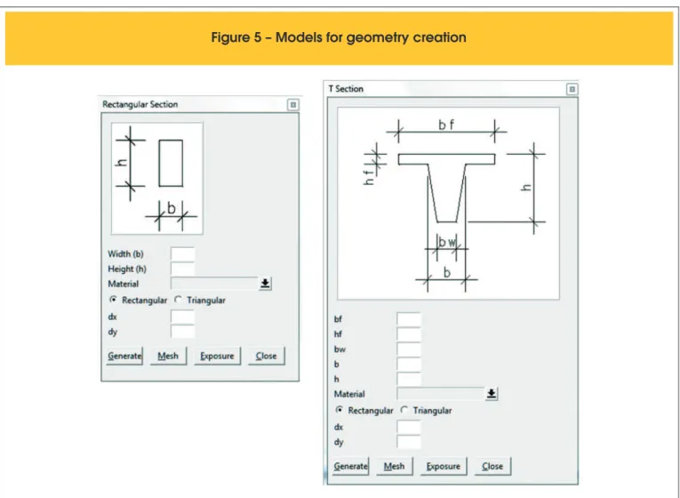
In order to ease the creation of the input data ile, some geometry

models, such as rectangular and T sections, were created based on GiD software [3], as shown in Figure 5. In these models, it is only necessary to inform the dimensions of the sections, of the

inite elements and the type of material.

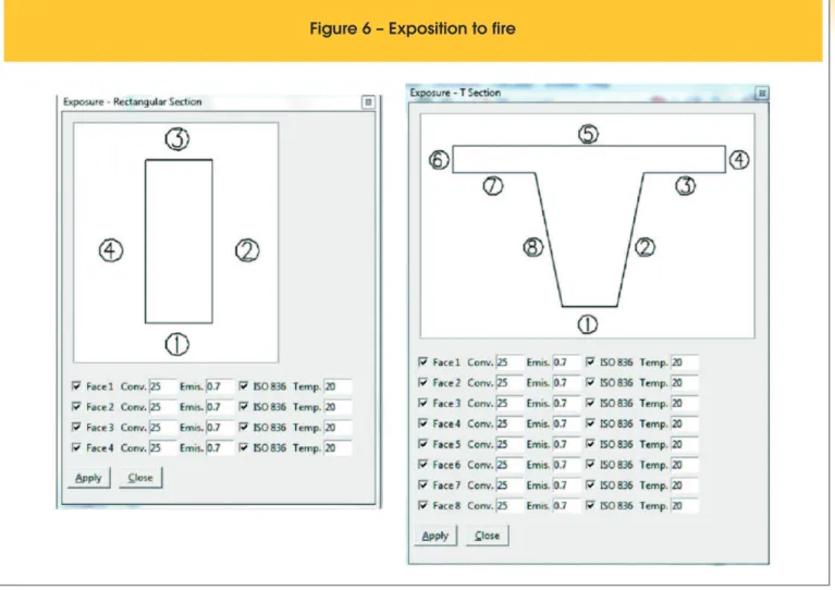
The exposition to ire can be conigured directly in the model, by the indication of the surfaces exposed to standard ire and

the surfaces exposed to a constant temperature, as shown in

Figure 6. In addition, emissivity and convection coeficients for the

consideration of heat transfer by convection and radiation should be informed.

The thermal properties of the materials, such as conductivity,

den-sity and coeficient of strength reduction, are informed by means of

tables in function of the temperature as shown in Figure 7. We can

also deine materials the thermal properties of which are indepen -dent of temperature.

Other data also necessary to the thermal analysis, such as total

time of ire exposition, time increment, initial temperature of the structure, α coeficient for the choice of the time integration method,

tolerance for temperatures convergence, time increase for printing

results, should be informed as shown in Figure 8. Coeficient α var -ies from 0 (Euler Implicit Method) to 1 (Euler Explicit Method) and

deines the numerical stability for the integration along time. STC software uses α=2/3, known as Galerkin Method.

5. Numerical simulation

In order to validate the software developed in this work, three simulations were performed, the results of which were compared to those obtained by means of STC [4] and ANSYS [6] software. The thermal properties adopted for concrete were based on ABNT NBR 15200.2012 [1]. In the examples herein, we used siliceous concrete humidity content equal to 1.5% in weight.

In all of the examples, the thermal action is determined according

to ISO 834 [8] standard ire curve.

5.1 Concrete beam

As example # 1, the heating of a 20 x 50 cm rectangular

(8)

Figure 6 – Exposition to fire

(9)

section concrete beam is analyzed, as shown in Figure 9. The ire is

admitted to act on three surfaces of the beam. The density of the con-crete is considered variable with temperature [1] and that for 20 ºC the density is equal to 2400 kg/m³, according to ABNT NBR 6118:2014

[9] recommendations. The emissivity factor and convection coeficient

were adopted equal to 0.7 and 25 W/m².ºC, respectively. For the initial temperature of the structure, the value 20ºC is adopted.

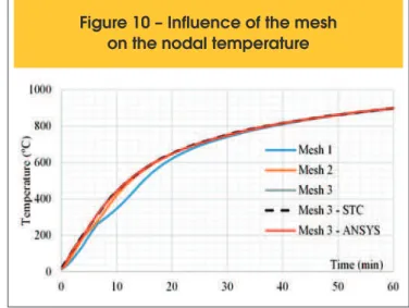
The structure was discretized in square elements. For ATERM soft-ware, 3 meshes were used: in Mesh 1, we used elements with 5 cm sides, in Mesh 2, with 2.5 cm sides and, in Mesh 3, with 1 cm sides. For modeling in ANSYS and STC, we only used Mesh 3.

Figure 10 shows the inluence of the mesh reinement on the evo -lution of temperature in function of time in the node in the middle of

the smaller heated side. With mesh reinement, the temperatures is observed to rise a little up to instant t = 28 minutes and after this

instant, the temperatures obtained for the different meshes are

vir-tually equal. The solution is veriied to tend to converge with mesh reinement and that, for Mesh 3, the results from ATERM, ANSYS

and STC are virtually equal.

5.2 Ribbed slab

Figure 11 shows the geometry of the thermally analyzed ribbed

slab (dimensions in cm). The slab underside is exposed to ire. The adopted values for emissivity factor and convection coefi -cient were 0.7 and 25 W/m².ºC, respectively, as per Eurocode 2 part 1.2 [5] recommendations. In the upside of the slab, not

exposed to ire, the combined phenomena of convection and ra

-Figure 8 – Other data

Figure 9 – Geometry of beam

Figure 10 – Influence of the mesh

on the nodal temperature

(10)

diation were simulated by αc = 9 W/m² °C [10]. The adopted initial structure temperature was 20 ºC. Due to symmetry, only half of the slab was modeled and the symmetry axis was considered to be adiabatic.

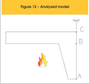
Figure 13 shows the variation in the nodal temperature in func-tion of time obtained by ATERM and STC for three distinct points located in the slab symmetry axis (as shown in Figure 12): point A – in the base of the rib. Point B – at the level of the junction between

the rib and the lange. Point C – in the upside of the slab. The slab

was discretized by triangular elements with 0.5 cm sides, 1653 ele-ments being generated in STC and 1809 eleele-ments in ATERM. The difference between the numbers of elements generated by the two pieces of software is due to the distinct mesh generators used by them. The results obtained from the two pieces of software are vir-tually equal. It is also noted that there is good correlation between the results from ATERM and ANSYS.

Figure 14 shows the ield of temperatures after 60 minutes of ire,

obtained by ATERM and STC.

5.3 Design of padded ribbed slabs

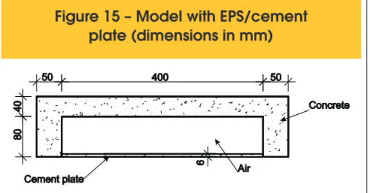
In Brazil, ribbed slabs illed with EPS on cement plates, as shown in

Figure 15, are also used. When heated, EPS decomposes

quick-ly, resulting in a large space illed with trapped air. This trapped

air contributes to the heat transfer between the cement plate,

which is at higher temperatures, and the lange. This heat trans -fer can be taken into account in the numerical model by means of the procedure indicated in item 3 herein.

In the face directly heated by the ire, we applied the ISO 834 [7]

standard curve and, in the face not directly exposed to the heat, a combination of convection and radiation, simulated by a_c = 9 W/

m² °C, was used.

The thermal properties of the cement plates used in the analyses

were: thermal conductivity equal to 2.22 W/mºC, speciic heat

equal to 840 J/kg K and density equal to 1200 kg/m³ [11]. The variation in temperature was analyzed in two points, as shown in Figure 16: point A – middle point of the upper face of the

lange and point B – located in the steel plate. EPS was admitted totally consumed by the ire and disregarded in the analysis.

The variation in temperature of points A and B, in function of the

Figure 13 – Temperature evolution

in function of time

! "#$% & #'(")*+,-.(/)0+1

(11)

time of ire exposition is represented in Figure 17. Once more,

a good correlation between the results obtained by ATERM and

STC is veriied.

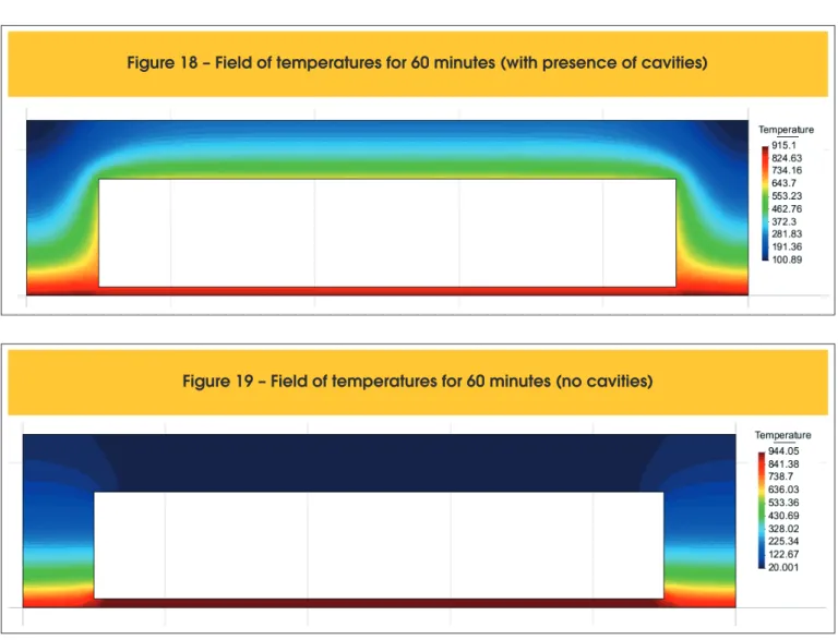
The consideration of the trapped air in the model is observed to cause heating in the upside of the slab in the region between ribs.

The ields of temperature at 60 minutes of standard ire on the

downside of the slab, with and without the trapped air consider-ation, are represented in Figures 18 and 19, respectively. Disregarding the air trapped inside the cavity does not generate the heating of the upside of the slab in the region between ribs,

i.e., after 60 minutes of ire, the upside of the slab is at room tem -perature. There is only a slight rise of the upside temperature in the region of the ribs.

In reality, the trapped air generates heat transfer by convection and radiation between the heated surface (the cement plate) and

the face not exposed to ire (lange). This example shows that this

heat transfer can be modeled by means of cavities.

6. Conclusion

Within this work, we presented the formulation of the Finite El-ement Method applied to non-linear thermal analysis of two-di-mensional structures, employed in the elaboration of the ATERM software. This kind of analysis is critical to the study of structures

in ire.

The results were validated with STC [4] and by means of ANSYS [6] software. It was observed that the results obtained by both types of software present an excellent correlation in all the ex-amples performed.

However, depending on the mesh used, the results were ob -served not to correspond to the physical behavior. Thus, a study of geometrical and time meshes is recommended before under-taking a thermal analysis.

In some situations, such as in ribbed slabs and ribbed slabs illed

with inert material, cavities do exist within the structural element.

Such cavities are illed with trapped air that, when heated, trans -fer heat by convection and radiation to the neighboring regions.

In the inite element analysis, the heat transfer by means of the

trapped air can be considered, both by ATERM and STC soft-wares.

The performance of ATERM showed that the software is very ef-fective in relation to STC, having a much shorter processing time. By means of the GiD software, several sections were created for data input, such as rectangular and T sections, which facilitate

the creation of the geometry and the mesh of inite elements.

Figure 15 – Model with EPS/cement

plate (dimensions in mm)

Figure 16 – Control points for the analysis

These basic models can be used to deine other more complex

geometries.

7. Acknowledgments

We thank FAPESP – the State of São Paulo Research

Founda-tion the Brazilian NaFounda-tional Council of Scientiic and Technological

Development, CNPq –and Tuper for their support.

8. Bibliography

[01] ASSOCIAÇÃO BRASILEIRA DE NORMAS TÉCNICAS. NBR 15200: Projeto de estruturas de concreto em situação de incêndio. Rio de Janeiro, 2012.

[02] PIERIN; I. A instabilidade de peris formados a frio em situ -ação de incêndio. Tese de Doutorado. Escola Politécnica. Universidade de São Paulo. 2011.

[03] International Center for Numerical Methods in Engineering (CIMNE). GiD 10.0 Users Manual. http://gid.cimne.upc.es/., 2011. [04] FIRE SAFETY DESIGN (FSD). TCD 5.0 User’s manual.

Lund: Fire Safety Design AB, 2007.

[05] EUROPEAN COMMITTEE FOR STANDARDIZATION. EN 1992-1-2: Eurocode 2: Design of concrete structures - part

1.2: general actions - actions on structures exposed to ire.

Brussels: CEN, 2004.

(12)