Lidar measurement of planetary boundary layer height and comparison with microwave profiling radiometer observation

(1)

AMTD

5, 1233–1251, 2012

Lidar measurement of planetary boundary layer

height

Z. Wang et al.

Title Page Abstract Introduction Conclusions References Tables Figures

◭ ◮

Back Close Full Screen / Esc

Printer-friendly Version

Discussion

P

a

per

|

Dis

cussion

P

a

per

|

Discussion

P

a

per

|

Discussio

n

P

a

per

Atmos. Meas. Tech. Discuss., 5, 1233–1251, 2012 www.atmos-meas-tech-discuss.net/5/1233/2012/ doi:10.5194/amtd-5-1233-2012

Atmospheric Measurement Techniques Discussions

This discussion paper is/has been under review for the journal Atmospheric Measurement Techniques (AMT). Please refer to the corresponding final paper in AMT if available.

Lidar measurement of planetary boundary

layer height and comparison with

microwave profiling radiometer

observation

Z. Wang1,2, X. Cao1, L. Zhang1, J. Notholt2, B. Zhou1, R. Liu1, and B. Zhang1

1

Key Laboratory for Semi-Arid Climate Change of the Ministry of Education, College of Atmospheric Sciences, Lanzhou University, Lanzhou, 730000, China

2

Institute of Environmental Physics, University of Bremen, 28334 Bremen, Germany Received: 18 January 2012 – Accepted: 25 January 2012 – Published: 7 February 2012 Correspondence to: L. Zhang (zhanglei@lzu.edu.cn)

(2)

AMTD

5, 1233–1251, 2012

height

Z. Wang et al.

◭ ◮

Printer-friendly Version Interactive Discussion

Discussion

P

a

per

|

Dis

cussion

P

a

per

|

Discussion

P

a

per

|

Discussio

n

P

a

per

|

Abstract

Using the wavelet technology method and lidar measurements the atmospheric bound-ary layer height was derived above the city of Lanzhou (China) and its suburb rural area – Yuzhong. Furthermore, at Yuzhong, the average boundary layer height and entrainment zone thickness was derived in convective situations. Simultaneously the 5

boundary layer height was derived from the microwave observations using a profiling radiometer and the parcel method. The results show that both data sets agree in strong convective situations. However, for weak convective situations the lidar measurements reveal boundary layer heights that are higher compared to the microwave observa-tions, because a decrease of the thermal boundary layer height does not directly lead 10

to a drop of aerosols in that altitude layer. Finally, the entrainment zone thicknesses are compared with theoretical predictions, and the results show some consistence be-tween both data sets.

1 Introduction

The boundary layer height (BLH) is a key parameter in describing the structure of 15

the atmospheric boundary layer (BL), it determines the volume available for pollutant dispersion. Currently, the BLH cannot be measured directly and it must be estimated from remote sensing profile measurements. The lidar remote sensing instrument is a useful tool to measure properties of the BL and the BLH.

Lidar backscattering measurements represent the relative concentration profiles of 20

atmospheric aerosols. Generally, most aerosols have their sources at the surface, producing high concentrations in the BL relative to the free atmosphere. There are usually sharp gradients in aerosol concentration at the BL top, this provides a method to determine the BLH.

Early lidar studies of BL used subjective visual estimates to determine the BLH, 25

(3)

AMTD

5, 1233–1251, 2012

height

Z. Wang et al.

◭ ◮

Discussion

P

a

per

|

Dis

cussion

P

a

per

|

Discussion

P

a

per

|

Discussio

n

P

a

per

and Eloranta, 1985), and identifications of the minimum in the vertical gradients of lidar profiles (Flamant et al., 1997) and maximum in variances of lidar signals (Hooper and Eloranta, 1986; Lammert and Boesenberg, 2006). The first of these suffer from the need to define appropriate threshold values, the second approach, the gradient one su_ffers from the e_ffects of noise and small-scale structure in the lidar profiles. Averaging 5

of the backscatter signal can minimize this problem but inevitably degrades the signal of interest. Steyn et al. (1999) presented an approach that fit an idealized profile to the observed one, another one widely used is based on the continuous wavelet transform method (Cohn and Angevineet, 2000; Davis et al., 2000; Brooks, 2003; Morille et al., 2007). When the vertical distribution of aerosols in the BL consists of a multi-layer 10

structure the lidar determination of the BLH will be complicated because it is not easy to determine a true BL top from these aerosols layer tops. The method applied in this article is based on the work of Morille et al. (2007). It differs from it in two aspects: (i) the multi-layer distribution of the aerosols is retrieved directly instead of single layer; (ii) a set of criterions is proposed to determine BLH from the evolution of multi-layer 15

structure, in which the continuity in evolution of BLH along time is a main consideration. The entrainment zone thickness is also an important parameter of the BL. An en-trainment zone locates at the top of the BL and consists of a mixture of air with the BL and free-troposphere characteristics. It is defined as the region with negative buoy-ancy flux, however various alternative definitions occur in measurements because of 20

different means (Boers et al., 1986; Nelson et al., 1989; Flamant et al., 1997; Cohn and Angevineet, 2000; Grabon et al., 2010). In this paper the method to find the locations of percentiles of BLH is applied, and the results are compared with that from theoretical models.

In the following, Sect. 2 introduces the sites and data, the method is described 25

(4)

AMTD

5, 1233–1251, 2012

height

Z. Wang et al.

◭ ◮

Discussion

P

a

per

|

Dis

cussion

P

a

per

|

Discussion

P

a

per

|

Discussio

n

P

a

per

|

2 Observation sites and instrumentation

The data used in this paper are from the Semi-Arid Climate Observatory and Labora-tory of Lanzhou University (SACOL) including two sites located at the suburb rural area of Lanzhou – Yuzhong (SACOL-Main) and the city of Lanzhou (SACOL-Lanzhou), re-spectively. At the city of Lanzhou a micro-pulse lidar (CE370-2) measures the aerosols 5

vertical profiles from ground to 30 km height with a time resolution of 30 min range resolution of 15 m. At Yuzhong, a microwave profiling radiometer (TP/WVP-3000) can obtain the vertical profiles of temperature, water vapor, and liquid water up to 10 km with a time resolution of 1 min and range resolution of 0.1 km for the height below 1 km and 0.25 km for 1–10 km. The fluxes of momentum, latent and sensible heat are 10

measured with a three-axis sonic anemometer (CSAT3) pointed into the prevailing wind direction, a micro-pulse lidar (MPL-4) records backscatter signals up to 20 km with a time resolution of 1 min and range resolution of 75 m.

3 Methodology

3.1 The detection of the BLH 15

The BLH is determined according to the sharp gradient of lidar profile at the top of the BL, however, the sharp gradient also occurs at the top of cloud or advected aerosols layer, which therefore should be identified firstly. The continuous wavelet transform (CWT) for each lidar profile is computed as

CWT_i(a, b)= Zz₂

z₁

p(z, t)g_i

_z

−b

a

1

√

adz, i=1, 2 (1)

20

g1(t)=(1−t2)e−t

2

/2_/p

2π (2)

g2(t)=−t e−t

2_/₂

(5)

AMTD

5, 1233–1251, 2012

height

Z. Wang et al.

◭ ◮

Discussion

P

a

per

|

Dis

cussion

P

a

per

|

Discussion

P

a

per

|

Discussio

n

P

a

per

where, p(z, t) represents the range-corrected backscatter. CWT₁(a, b) has its mini-mum at the top and base of cloud or advected aerosols layer and maximini-mum at their peaks. After determining some possible particles layers, a threshold value thre1 is ap-plied. These satisfying∆p=p(zpeak,t)−p(zbase,t)>thre1 are considered to be true.

Similarly, CWT2(a, b) has its maximum at the part of lidar profile where the

range-5

corrected backscatter decreases with height. The largest maximum of CWT2(a, b)

often occurs at the top of the BL when both cloud and advected aerosols layer are absent. Currently the following method is applied to retrieve the BLH.

– The first, second and third largest values (H1, H2, H3) are selected from the maximums of CWT2(a, b) except for ones corresponding to the top of cloud or

10

advected aerosols layer. In cloudy situations, only these maximums with locating under the base of the cloud are considered. The locations of the three maximums denote likely BL top.

– oldblh is defined as the average of five successive BLHs with their time before present lidar profile’s and the variation of each of them relative to the earlier one 15

all smaller than a threshold thre2. Then, following rules are applied.

1. In cloudless situations, if there is an advected aerosols layer and all maximums of CWT2(a, b) locating under the base of this aerosol layer are smaller than a

threshold thre3, then the one closer to the oldblh between its top and base will be 20

considered as the BL top.

(6)

AMTD

5, 1233–1251, 2012

height

Z. Wang et al.

◭ ◮

Discussion

P

a

per

|

Dis

cussion

P

a

per

|

Discussion

P

a

per

|

Discussio

n

P

a

per

|

3. If both (1) and (2) do not match, there is neither cloud nor advected aerosols layer andH1 is smaller than thre4, then the earlier BLH will be considered as a present one.

4. If (1), (2) and (3) do not match, the following functions will be applied,

r(x)=mine−x−σc(t),₁

(4) 5

ratio=H/H1 (5)

where,c(t)=minA1−A2

A3 t+A2, A1

represents a range in which the difference be-tween two successive BLHs seems reasonable andσ=c(t)/5 ln 2. A₁,A₂andA₃ are some empirical parameters andtrepresents time.H represents a one whose height is closer to oldblh betweenH2 andH3.r(_|z_H1−oldblh|) characterizes a

de-10

gree to which the height of theH1 denotes the true BLH and ratio characterizes a reverse one. If ratio is larger thanr(_|zH1−oldblh|), then the location ofH will be

considered as the BL top, otherwise the location ofH1 is accepted. This criterion guarantees the temporal continuity of development of the BLH. The parameters in the expressions above vary according to the time resolution of lidar data, the 15

larger the interval between two successive records is, the less important it is.

3.2 Average BLH and entrainment zone thickness

A single lidar profile from MPL-4 represents an average for one minute measurements and the BLH from the single profile denotes local BLH, so average BLH and entrain-ment zone thickness can be derived from its time sequence. Firstly, calculate a cumu-20

(7)

AMTD

5, 1233–1251, 2012

height

Z. Wang et al.

◭ ◮

Discussion

P

a

per

|

Dis

cussion

P

a

per

|

Discussion

P

a

per

|

Discussio

n

P

a

per

of the value corresponding to 10 %, 90 % and 50 % of CPD and that of the second-order polynomial. At the same time, the BLH is also obtained from temperature profile of TP/WVP-3000 by parcel method (Holzworth, 1964).

3.3 Parameterization theory of entrainment zone thickness

According to parcel theory the entrainment zone thickness is related to the kinetic en-5

ergy and resistance of the air parcel rising (Bores and Eloranta, 1986), and can be writ-ten as:_∆h∝_g_∆w_θ/θ2

0

, where_∆his the entrainment zone thickness,gis the gravitational constant,∆θis the potential temperature jump across the entrainment zone,θ0is the

average potential temperature in the BL,wis the vertical velocity usually characterized by the convective velocity scale defined as: w_∗3=g(w′θ′)sh

θ₀ , wherehis the average BLH, 10

(w′_θ′₎_s_{is the kinematic heat flux at the surface. Gryning et al. (1994) derived another}

parameterization theory based on the turbulent-kinetic-energy equation. It can be writ-ten as: ∆_hh_∝(RiE)−

1/3

, where RiE=

(g/θ0)h∆θ

w2 e

is the entrainment Richardson number, we=∂h_∂t −wLis the entrainment velocity,wLis large-scale mean vertical velocity, which

can be neglected in case of strong convection. In addition, ∆_hh∝

_w e

w_∗

α

was proposed 15

by Nelson et al. (1989), where three possible exponents 1.0, 0.5 and 0.25 are sug-gested. The retrieved entrainment zone thickness is examined through these theories, the kinematic heat flux at the surface is provided by the three-axis sonic anemometer, the mean potential temperature of the BL and potential temperature jump are derived from temperature profile by the microwave profiling radiometer. However, there may be 20

(8)

AMTD

5, 1233–1251, 2012

height

Z. Wang et al.

◭ ◮

Discussion

P

a

per

|

Dis

cussion

P

a

per

|

Discussion

P

a

per

|

Discussio

n

P

a

per

|

4 Results

4.1 Meteorological conditions on Lanzhou

– 28 January 2007: clear sky throughout the whole day.

– 7 January 2007: cirrus coverage of 90 % from 08:00 CST to 17:00 CST, fair weather during the rest of the day.

5

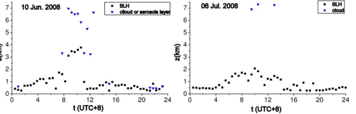
– 6 July 2008: clear sky throughout the whole day. – 10 June 2008: almost clear throughout the whole day.

4.2 The BL in the city of Lanzhou

Figures 1 and 2 show lidar observations performed in the city of Lanzhou. Lanzhou is located in a valley basin. The basin is elliptical, surrounded by mountains with the 10

Yellow River flowing across the city. The geography makes it di_fficult for pollutants to diffuse. The vertical distributions of aerosols in the BL usually show a complicated multi-layer structure. Figure 1 shows the evolution of the heights ofH1,H2 andH3 to illustrate this distinguishing feature. On 28 January 2007, onlyH2 and H3 larger than 0.15H1 have been showed, and 0.25H1 on 7 January 2007.

15

On 28 January 2007, the aerosols concentrations for the whole day below 0.5 km are relatively high compared to the ones above 0.5 km. There are very strong gradients in aerosols concentration at the top of the aerosols layer, and H1 mainly denotes its top. After 09:00, the thermal rising of the air-masses produce another aerosol layer with weak gradients at its top above the first one, H2 denotes its top before 16:00. 20

(9)

AMTD

5, 1233–1251, 2012

height

Z. Wang et al.

◭ ◮

Discussion

P

a

per

|

Dis

cussion

P

a

per

|

Discussion

P

a

per

|

Discussio

n

P

a

per

It is difficult to determine the correct BLH in most cases owing to the multi-layer distributions of aerosols in the city of Lanzhou, so it seems more advisable that the heights ofH1,H2 andH3 are give together, as in Fig. 1.

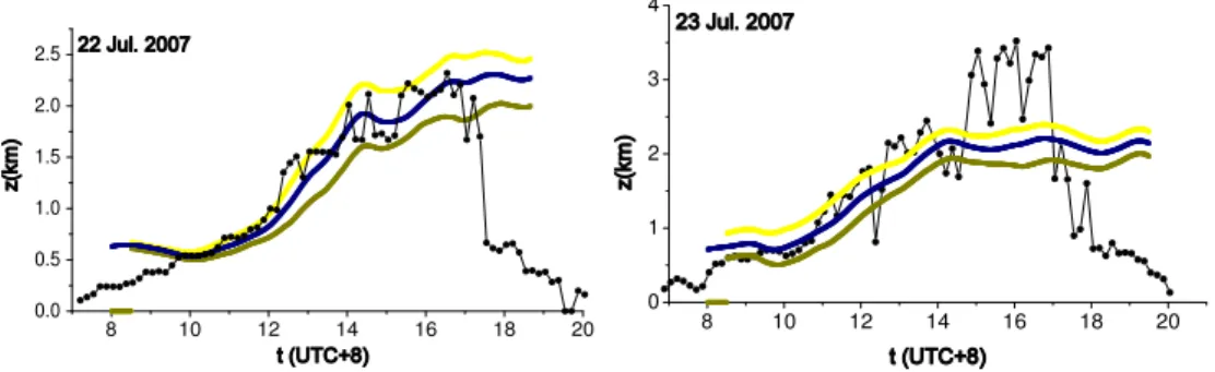
4.3 The BL in suburb rural area of Lanzhou – Yuzhong

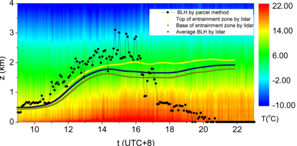
Figure 3 shows the results from lidar and microwave profiling radiometer measure-5

ments on 29 July 2007 at SACOL. Between 11:00 and 16:00 the BLH from lidar are about 0.5 km smaller than the ones from microwave profiling radiometer and the latter begin to rise rapidly from 11:00 while the results from the lidar increase more slowly. After 16:00, the BLH retrieved by the parcel method reduce quickly and disappear at 20:00, but results from lidar maintain at heights of 2.0 km. This discrepancy is caused 10

by the fact that the BLH retrieved by the parcel method represents an up limit height that the rising thermal air-masses can reach while that from lidar observation repre-sents the height of the aerosols layer, aerosols do not drop immediately even if the up limit height decreases.

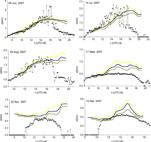
Figure 4 shows results for six measurement days in the period of June to Decem-15

ber 2007. In situations with strong convection, the BLH from lidar agrees with that from profiling radiometer measurements, such as the examples in June, July and August show. However, in situations with weak convection, the BLH from lidar is markedly higher, as shown by the observations in September, November and December.

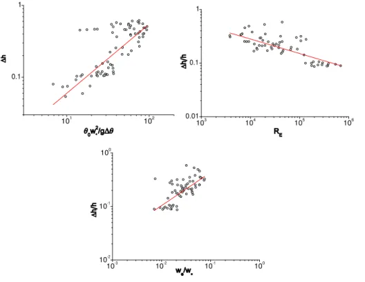
4.4 Examination of entrainment zone thickness by parameterization theory 20

(10)

AMTD

5, 1233–1251, 2012

height

Z. Wang et al.

◭ ◮

Discussion

P

a

per

|

Dis

cussion

P

a

per

|

Discussion

P

a

per

|

Discussio

n

P

a

per

|

In Fig. 6 the expression fitted according to the parcel theory is

∆h=0.0065

w_∗2 g∆θ/θ₀

0.96

, the correlation coefficient is R2=0.59 using 74 data

points. The result following Bores et al. (1986) is ∆h=38.41

w_∗2 g∆θ/θ0

0.41

. The

ex-pression based on the theory proposed by Gryning et al. (1994) is ∆_hh=3.38 (RiE)− 0.27

, here correlation coefficientR2=0.56 using 62 data points. The result derived by Gryn-5

ing et al. (1994) is ∆_hh=3.3 (RiE)− 1/3

+0.2. The last fitted relation is ∆_hh=1.8we

w_∗

0.62

, where the correlation coefficient isR2=0.49 for 62 data points.

5 Conclusions

The BLH over the city of Lanzhou and its suburb rural area – Yuzhong has been ob-tained using a modified wavelet technology and lidar data. The results reveal the 10

effectiveness of this method. At Yuzhong, the BLH is also calculated using data of microwave profiling radiometer. The comparison shows that both data sets agree un-der strong convective conditions when the BL grows. However, unun-der conditions with weak convection the lidar data reveal higher values for the BLH. Further, in the case of Yuzhong the entrainment zone thickness is derived from the BLH. The comparison 15

between measured quantity and that predicted by several theories reveals that some consistence exists in them but the di_fference is also obvious.

Some characteristics about the BL can be concluded from these results. The BLH above the city of Lanzhou often maintains at about 0.5 km throughout the whole day without significant development in winter. At Yuzong, the largest height the BL can 20

(11)

AMTD

5, 1233–1251, 2012

height

Z. Wang et al.

◭ ◮

Discussion

P

a

per

|

Dis

cussion

P

a

per

|

Discussion

P

a

per

|

Discussio

n

P

a

per

An ideal condition for a lidar to retrieve the BLH is that the lower atmosphere can be divided into three parts according to the aerosols distribution, the BL with much aerosols and tiny variation in aerosols concentration, the entrainment zone with pro-nounced drop in aerosols concentration and free atmosphere with little aerosols. So the BLH from the lidar represents a surface-based aerosol layer’s depth and does not 5

necessarily agree with the one defined by thermodynamics and dynamic properties of the BL.

Clouds have a great impact on the results of the BLH derived by the lidar. For the nascent clouds with strong gradients in the lidar signals at their tops, but without af-firmed cloud characteristics, the above-mentioned algorithm likely reveals their tops as 10

those of the BL. Sometimes the lidar profiles will be disorderly preventing the retrieval of useful information when boundary layer clouds are dissipating. Moreover, false BLH maybe appear owing to the remanent vapors.

Convection boundary layer begins to grow after sunrise, however, it is di_fficult for a lidar to capture its top before it grows beyond the nocturnal boundary layer.

15

Acknowledgements. The research is supported by the National Important Science Research

Program of China (2012CB955302) and the National Natural Science Foundation of China (41075104). We gratefully thank the Semi-Arid Climate Observatory and Laboratory of Lanzhou University providing observation data.

References 20

Baars, H., Ansmann, A., Engelmann, R., and Althausen, D.: Continuous monitoring of the boundary-layer top with lidar, Atmos. Chem. Phys., 8, 7281–7296, doi:10.5194/acp-8-7281-2008, 2008.

Boers, R. and Eloranta, E. W.: Lidar measurements of the atmospheric entrainment zone and the potential temperature jump across the top of the mixed layer, Bound.-Lay. Meteorol., 34,

25

(12)

AMTD

5, 1233–1251, 2012

height

Z. Wang et al.

◭ ◮

Discussion

P

a

per

|

Dis

cussion

P

a

per

|

Discussion

P

a

per

|

Discussio

n

P

a

per

|

Cohn, S. A. and Angevine, W. M.: Boundary layer height and entrainment zone thickness measured by lidars and wind-profiling radars, J. Appl. Meteorol., 39, 1233–1247, 2000. Davis, K. J., Gamage, N., Hagelberg, C. R., Kiemle, C., Lenschow, D. H., and Sullivan, P. P.:

An objective method for deriving atmospheric structure from airborne lidar observations, J. Atmos. Ocean Tech., 17, 1455–1468, 2000.

5

De Haij, M., Wauben, W., and Bltink, H. K.: Determination of mixing layer height from ceilometer backscatter profiles, Royal Netherlands Meteorological Institute, P.O. Box 201, 3730 AE De Bilt, The Netherlands.

Emeis, S. and Schafer, K.: Remote sensing methods to investigate boundary-layer structures relevant to air pollution in cities, Bound.-Lay. Meteorol., 121, 377–385, 2006.

10

Emeis, S., Muenkel, C., Vogt, S., Mueller W. J., and Schaefer, K.: Atmospheric boundary-layer structure from simultaneous SODAR, RASS, and ceilometer measurements, Atmos. Environ., 38, 273–286, 2004.

Emeis, S., Schaefer, K., and Muenkel, C.: Surface-based remote sensing of the mixing-layer height – a review, Meteorol. Z., 17, 621–630, 2008a.

15

Emeis, S., Schafer, K., and Munkel, C.: Long-term observations of the urban mixing-layer height with ceilometers, 14th international symposium for the advancement of boundary layer remote sensing, 2008b.

Flamant, C., Pelon, J., Flamant, P. H., and Durand, P.: Lidar determination of the entrainment zone thickness at the top of the unstable marine atmospheric boundary layer, Bound.-Lay.

20

Meteorol., 83, 247–284, 1997.

Grabon, J. S., Davis, K. J., Kiemle, C., and Ehret, G.: Airborne lidar observatrions of the transition zone between the convective boundary layer and free atmosphere during the in-ternational H₂O project (IHOP) in 2002, Bound.-Lay. Meteorol., 134, 61–83, 2010.

Gryning, S. E. and Batchvarova, E.: Parameterization of the depth of the entrainment zone

25

above the daytime mixed layer, Q. J. Roy. Meteor. Soc., 120, 47–58, 1994.

Holzworth, C. G.: Estimates of mean maximum mixing depths in the contiguous United states, Mon. Weather Rev., 92, 235–242, 1964.

Hooper, W. P. and Eloranta, E.: Lidar measurements of wind in the planetary boundary layer: the method, accuracy and results from joint measurements with radiosonde and kytoon, J.

30

Clim. Appl. Meteorol., 25, 990–1001, 1986.

(13)

AMTD

5, 1233–1251, 2012

height

Z. Wang et al.

◭ ◮

Discussion

P

a

per

|

Dis

cussion

P

a

per

|

Discussion

P

a

per

|

Discussio

n

P

a

per

Morille, Y., Haeffelin, M., Drobinski, P., and Pelon, J.: STRAT: an automated algorithm to retrieve the vertical structure of the atmosphere from single-channel lidar data, J. Atmos. Ocean. Tech., 24, 761–775, 2007.

Nelson, E., Stull, R. B., and Eloranta, E.: A prognostic relation for entrainment zone thickness, J. Appl. Meteorol., 28, 885–903, 1989.

5

Seibert, P., Beyrich, F., Gryning, S.-E., Sylvain, J., Rasmussen, A., and Tercier, P.: Review and intercomparison of operational methods for the determination of the mixing height, Atmos. Environ., 34, 1001–1027, 2000.

Steyn, D., Baldi, M., and Hoff, R. M.: The detection of mixed layer depth and entrainment zone thickness from lidar backscatter profiles, J. Atmos. Ocean Tech., 16, 953–959, 1999.

10

Stull, R. B.: An Introduction to boundary Layer Meteorology, Kluwer Academic Publishers, Dordrecht/Boston/London, 1988.

(14)

AMTD

5, 1233–1251, 2012

height

Z. Wang et al.

◭ ◮

Discussion

P

a

per

|

Dis

cussion

P

a

per

|

Discussion

P

a

per

|

Discussio

n

P

a

per

|

0 4 8 12 16 20 24

0.0 0.5 1.0 1.5 2.0 2.5 3.0

0 4 8 12 16 20 24

0 1 2 3 4 5 6 7

(15)

AMTD

5, 1233–1251, 2012

height

Z. Wang et al.

◭ ◮

Discussion

P

a

per

|

Dis

cussion

P

a

per

|

Discussion

P

a

per

|

Discussio

n

P

a

per

0 4 8 12 16 20 24

0 1 2 3 4 5 6 7

0 4 8 12 16 20 24

0 1 2 3 4 5 6 7

(16)

AMTD

5, 1233–1251, 2012

height

Z. Wang et al.

◭ ◮

Discussion

P

a

per

|

Dis

cussion

P

a

per

|

Discussion

P

a

per

|

Discussio

n

P

a

per

|

(17)

AMTD

5, 1233–1251, 2012

height

Z. Wang et al.

◭ ◮

Discussion

P

a

per

|

Dis

cussion

P

a

per

|

Discussion

P

a

per

|

Discussio

n

P

a

per

(18)

AMTD

5, 1233–1251, 2012

height

Z. Wang et al.

◭ ◮

Discussion

P

a

per

|

Dis

cussion

P

a

per

|

Discussion

P

a

per

|

Discussio

n

P

a

per

|

8 10 12 14 16 18 20 0.0

0.5 1.0 1.5 2.0 2.5

8 10 12 14 16 18 20 0

1 2 3 4

(19)

AMTD

5, 1233–1251, 2012

height

Z. Wang et al.

◭ ◮

Discussion

P

a

per

|

Dis

cussion

P

a

per

|

Discussion

P

a

per

|

Discussio

n

P

a

per

101 102

0.1 1

103 104 105 106

0.01 0.1 1

10-3 10-2 10-1 100

10-2 10-1 100