www.ann-geophys.net/28/825/2010/
© Author(s) 2010. This work is distributed under the Creative Commons Attribution 3.0 License.
Annales
Geophysicae
Elastic-backscatter-lidar-based characterization of the convective
boundary layer and investigation of related statistics
S. Pal, A. Behrendt, and V. Wulfmeyer
Institute of Physics and Meteorology (IPM), University of Hohenheim, Garbenstrasse 30, 70599 Stuttgart, Germany Received: 23 February 2009 – Revised: 5 January 2010 – Accepted: 11 March 2010 – Published: 22 March 2010
Abstract. We applied a ground-based vertically-pointing aerosol lidar to investigate the evolution of the instantaneous atmospheric boundary layer depth, its growth rate, associ-ated entrainment processes, and turbulence characteristics. We used lidar measurements with range resolution of 3 m and time resolution of up to 0.033 s obtained in the course of a sunny day (26 June 2004) over an urban valley (cen-tral Stuttgart, 48◦47′N, 9◦12′E, 240 m above sea level). The lidar system uses a wavelength of 1064 nm and has a power-aperture product of 2.1 W m2.
Three techniques are examined for determining the in-stantaneous convective boundary layer (CBL) depth from the high-resolution lidar measurements: the logarithm gra-dient method, the inflection point method, and the Haar wavelet transform method. The Haar wavelet-based ap-proach is found to be the most robust technique for the au-tomated detection of the CBL depth. Two different regimes of the CBL are discussed in detail: a quasi-stationary CBL in the afternoon and a CBL with rapid growth during morn-ing transition in the presence of dust layers atop. Two dif-ferent growth rates were found: 3–5 m/min for the grow-ing CBL in the morngrow-ing and 0.5–2 m/min durgrow-ing the quasi-steady regime. The mean entrainment zone thickness for the quasi-steady CBL was found to be∼75 m while the CBL top during the entire day varied between 0.7 km and 2.3 km. A fast Fourier-transform-based spectral analysis of the instanta-neous CBL depth time series gave a spectral exponent value of 1.50±0.04, confirming non-stationary CBL behavior in the morning while for the other regime a value of 1.00±0.06 was obtained indicating a quasi-stationary state of the CBL.
Assuming that the spatio-temporal variation of the particle backscatter cross-section of the aerosols in the scattering vol-ume is due to number density fluctuations (negligible
hygro-Correspondence to:S. Pal ([email protected])
scopic growth), the particle backscatter coefficient profiles can be used to investigate boundary layer turbulence since the aerosols act as tracers. We demonstrate that with our lidar measurements, vertical profiles of variance, skewness, and kurtosis of the fluctuations of the particle backscatter co-efficient can be determined. The variance spectra at differ-ent altitudes inside the quasi-steady CBL showed anf−5/3 dependency. The integral scale varied from 40 to 90 s (de-pending on height), which was significantly larger than the temporal resolution of the lidar data. Thus, the major part of the inertial subrange was detected and turbulent fluctuations could be resolved. For the quasi-stationary case, negative values of skewness were found inside the CBL while posi-tive values were observed in the entrainment zone near the top of the CBL. For the case of the rapidly growing CBL, the skewness profile showed both positive and negative values even inside the CBL.
Keywords. Atmospheric composition and structure (Aerosols and particles) – Meteorology and atmospheric dynamics (Convective processes; Turbulence)
1 Introduction
Monitoring of the atmospheric boundary layer (ABL) is an important issue in atmospheric science since this layer is in-fluenced by both the strength of land-surface exchange at the bottom and of entrainment processes at the top. These pro-cesses control the transport of particles, trace gases, and heat between the ground and the free troposphere (Stull, 1988).
and therefore, the ABL depth is variable on short time scales. According to Stull (1988), the ABL depth is defined as the “average height of the inversion base”. In contrast to this def-inition of a mean ABL depth, appropriate observational data with high temporal resolution allow to identify an instanta-neous ABL depth and suggest studies on its variability.
The top of the ABL (here onwards referred as ABL height) can also be defined as the height of the minimum sensible heat flux. As long as passive scalars are accumulated in the ABL without the presence of any residual layer (RL) or aerosol layer (AL), large gradients of aerosol concentra-tion or water vapor density occur at the inversion capping the ABL. These gradients are also suited for defining the top of the ABL (Stull, 1988). In ideal cases, the location of these gradients coincides with the minimum in the buoyancy flux profile (Sullivan et al., 1998). A sharp potential temperature jump also determines the ABL top (Boers et al., 1984). In consequence, the ABL height can be identified by character-istic features in profiles of several atmospheric variables. The most conventional method uses radiosonde-measured pro-files of wind, temperature, and relative humidity (RH). It is noteworthy, that this approach yields a “snapshot”-view of the atmosphere. In contrast to radio soundings, active re-mote sensing systems are capable of providing continuous measurements of the key-variables of the atmosphere with high spatial and temporal resolution leading to better sam-pling statistics of the instantaneous ABL height. For this purpose, sodar (e.g. Beyrich and Gryning, 1998), radar wind profiler (e.g. Angevine et al., 1994), and lidar system (e.g. Russel et al., 1974) are in use. All these approaches have specific shortcomings and measurement uncertainties (Seib-ert et al., 2000).
In principle, determination of the ABL height with elas-tic backscatter lidar uses one of the following two methods: either a variance-based analysis through observation of mix-ing processes in the ABL or a gradient-based analysis of the vertical distribution of a passive tracer. For instance, the variance profile allows determining the mean convectively-driven atmospheric boundary layer (CBL) top height (hence-forth referred as CBL height). The variance technique has been recently used by Lammert and B¨osenberg (2006) to confirm the results of the logarithm gradient method (LGM), the most simple gradient approach. Also Martucci et al. (2007) compared the results obtained from LGM and the variance method but found that the mean CBL heights com-puted by LGM are statistically higher than the CBL heights computed by the variance method.
Previous lidar studies (e.g., Kiemle et al., 1997; Menut et al., 1999; Davis et al., 2000; Brooks, 2003; Wulfmeyer and Janji´c, 2005; He et al., 2006) used one or two of three dif-ferent gradient-based techniques for the ABL height deter-mination: LGM, inflection point method (IP), and the Haar wavelet transform (HWT) scheme. In this article, we start the analyses with a comparison of CBL height retrievals via all three gradient-based techniques that have been used within
the literature so far and compare the results with higher-order moment analyses including variance-based method to deter-mine the ABL height.
The comparison of LGM, IP and HWT is a worthwhile en-deavor, since the various approaches used to determine CBL depth, generally produce slightly different results, and under-standing of how they differ is necessary to compare different studies. To the best of our knowledge, no such study has been carried out yet. We apply these three techniques for the CBL height determination to very high resolution lidar measure-ments of 3 m and 0.33 s.
Once the evolution of the CBL height is determined with the best available approach, it is interesting to study whether these time series can help to quantify the non-stationarity involved. Major challenges lie in the application of a suit-able approach to the problem of non-stationarities of the CBL height evolution. This arises due to the presence of vigorous thermal up- and downdrafts in this region. The CBL consists of highly fluctuating and irregular structures. Therefore, the top of the CBL is an implicative of this fluctuation. In or-der to quantify the aspects of variability and correlations at different temporal and spatial scales, fast Fourier transforma-tion (FFT)-based power spectral analysis has been applied to the time series of instantaneous CBL height.
Smaller-scale processes often become important in the en-trainment zone (EZ) due to high variability in the distribu-tion of aerosol particles in these regions. The EZ is basically that region near the top of the boundary layer where vigorous mixing of the free-tropospheric air (by downdraft) and the thermals (by updraft) of the CBL occurs (Stull, 1988). Esti-mation of the entrainment zone thickness (EZT) therefore re-quires very high tempo-spatially resolved information of the tracers in this region. The instantaneous CBL height can sig-nificantly change within short time intervals especially when the convective activity is strong. The very high spatial res-olution of lidar data yields an opportunity which is unique among all remote sensing techniques to capture small-scale features.
(Senff et al., 1996, among others) for investigating the turbu-lence features in the CBL. Recently, Engelmann et al. (2008) used lidar measurements of aerosol backscatter to estimate the aerosol flux in a CBL. However, in this study, the ver-tical profiles of higher-order moments of aerosol backscat-ter were not debackscat-termined. The temperature gradient, which the definition of ABL height is based on, can be measured with rotational Raman lidar (Behrendt, 2005). Comparisons of LGM-determined CBL top values with such lidar-based temperature measurements have been presented by Radlach et al. (2008).
Statistical results of higher-order moments analyses of the particle backscatter signals inside the boundary layer are of high interest in order to explore the stochastic nature of tur-bulence. Indeed, these moments describe the tails of the probability density function; in particular, they provide the degree of the departure from a Gaussian form. The vertical profiles of these moments in the CBL provide further knowl-edge to foster our understanding about CBL turbulence fea-tures.
The aerosol lidar system of University of Hohenheim (UHOH) was installed in downtown Stuttgart to acquire data on four days from 23 to 26 June 2004. The primary objective for using the UHOH lidar was to obtain a close picture of the depth and variability of the CBL in this region and the con-sequent understanding of the CBL processes during different times of a day in summer. Such an experiment to explore the details of the CBL has not been made before in this area.
This paper is organized as follows. A brief description of the experimental site and meteorological conditions is given in Sect. 2. The set up of the UHOH lidar system is introduced in Sect. 3. The three gradient methods to determine the CBL height and the techniques to determine EZT and higher-order moments are outlined in Sect. 4. The results of the two cases are discussed in Sect. 5. A brief summary and an outlook are presented in Sect. 6.
2 The experimental site and meteorological conditions
The UHOH lidar system was deployed during the measure-ment period near the center of Stuttgart (48◦46′43.5′′N, 9◦10′48.9′′E, elevation approximately 240 m above sea level, a.s.l.) in southwestern Germany. The experimental site is located in a valley with complex topography. It is characterized by a large population density, high density of buildings, diverse anthropogenic activities, non-uniform land use, and enhanced industrial activities. Stuttgart is a major transportation cross point, including a large river port, an in-ternational airport, and a considerable industrial center. The orography of this city with the deepest point at the Neckar river of about 200 m a.s.l. and the highest point in Stuttgart-Vaihingen of about 550 m a.s.l. (just a few km away) influ-ences the meteorological conditions.
Table 1. Technical parameters of the vertically-pointing UHOH elastic aerosol lidar system.
Transmitter Nd:YAG laser
Wavelength: 1064 nm
Pulse energy: 600 mJ @1064 nm Pulse repetition rate: 30 Hz
Pulse duration: 10 ns Power aperture product: 2.12 Wm2
Telescope
Type: Ritchey-Chretien (Astro
Optic) Diameter of primary mirror: 40 cm Diameter of secondary mirror: 10 cm
Focal ratio: f/10
Coating: Aluminum with quartz
protective coating
Detectors Si-APD for 1064 nm and PMT for 532 nm
Analog-to-digital converter
Compu-Scope 14 100
Analog-to-digital resolution: 14 bits
Sampling rate: 50 Ms/s (for 2 channels) Sampling in range: 3 m
During the measurement period, the sky was mostly cloud-free. As to weather conditions, absolute maximum tempera-ture of 25.5◦C, absolute minimum of 9.5◦C, maximum RH of 78.4% and minimum of 16.2% RH at ground, only fair weather cumuli, some thin cirrus clouds and no precipita-tion were observed during the measurement period. The mean wind speed at 10 m height was 3–4 ms−1. This me-teorological dataset was collected by the weather station in Stuttgart City (Amt f¨ur Umweltschutz der Stadt Stuttgart, Schwabenzentrum-Stadtmitte, at 48◦46′20′′N, 9◦10′46′′E,
275 m a.s.l.) about 500 m distant from the lidar site. The surface temperature on 26 June 2004 reached its maximum value of 25.5◦C at 16:30 CEST (central European summer time, UTC+2 h). Horizontal wind obtained at 10 m height was mild (1–1.5 ms−1). The RH at ground showed a classical diurnal cycle with a maximum RH of about 80% at around 06:00 CEST and minimum RH of 30% at 17:00 CEST on 26 June 2004. The UHOH lidar continuously monitored the CBL for more than eight hours on this day. Consequently, within this study, we decided to use the lidar measurements obtained on this day.
3 Experimental set up of the lidar system
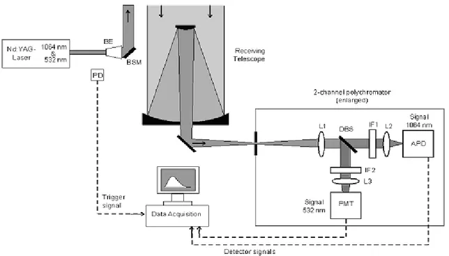
Fig. 1. Scheme of the elastic backscatter lidar of UHOH. APD: Avalanche photodiode, BE: Beam expander, BSM: Beam steering mirror, DBS: Dichroic beam splitter, IF1–IF2: Interference filters, L1–L3: Lenses, PMT: Photomultiplier tube, PD: Photodiode.
for aerosol and temperature measurements (Behrendt et al., 2005; Pal et al., 2006, 2010; Radlach et al., 2008).
This version of the lidar system worked in monostatic vertically-pointing biaxial configuration with a maximum spatial and temporal resolution of 3 m and 0.033 s, respec-tively. The lidar system was equipped with a flash-lamp-pumped Nd:YAG laser emitting simultaneously the funda-mental and the second harmonic wavelengths of 1064 nm and 532 nm, respectively. Pulses of∼10 ns duration with a pulse energy of 600 mJ at both wavelengths were transmitted. The schematic set-up and specifications of the lidar system are shown in Fig. 1 and Table 1, respectively.
The backscattered light was sampled with a Ritchey-Chretien-type telescope with a 40-cm-diameter primary mir-ror. The backscattered light passed a lens and was then split by a dichroic beam splitter, separating the signals of the two transmitted wavelengths. The two beams were analyzed by means of two interference filters, both with 5 cm diameter and 10 nm half-width-at-half-maximum (HWHM) band-pass before reaching the detectors: a photomultiplier tube (PMT, Hamamatsu R7400-U02) for 532 nm and a silicon avalanche photodiode (Si-APD, Perkin & Elmer C3095E) for 1064 nm. The diameter of the sensitive area of the APD and the PMT were 0.8 mm and 8 mm, respectively.
The data acquisition system stored the lidar data with a frequency of 30 Hz, i.e., for each laser pulse. The data acqui-sition and processing unit was comprised of a two-channel Gage CS 14100 card with 14 bit resolution analog-to-digital converter sampling the backscattered signal with 50 MHz to
provide data with 3 m vertical resolution, and a standard per-sonal computer. It processed the lidar data using an auto-mated LabView code and then stored on a hard disk. The vertical profiles of the raw and the range-square-corrected backscatter signal and time-versus altitude images of the li-dar signal were displayed in real time.
4 Methods
4.1 Determination of the atmospheric boundary layer height
4.1.1 Lidar equation
The monostatic elastic lidar signal is expressed as
Pλ(R)=P0,λ
ctp
2 Keff A
R2O (R)βλ(R)exp
−2
R
Z
0
αλ(r)dr
.
(1) where Pλ(R) is the received signal intensity at the
wave-length λ from range R,P0,λ is the laser peak power, c is
the velocity of light, tp is the laser pulse duration, Keff is the overall efficiency of the lidar system, A is the receiv-ing area of the telescope, O(R)is the laser-beam receiver-field-of-view overlap function,βλ(R)is the total backscatter
coefficient due to atmospheric particles and molecules, and αλ(R) is the total extinction coefficient due to atmospheric
at 1064 nm, the range-square-corrected backscatter signal in-tensity is approximately proportional to the particle backscat-ter coefficient (βλ,par); the Rayleigh scattering due to the at-mospheric molecules at this wavelength is nearly negligible. In this case, Eq. (1) can be approximated as
Pλ(R) R2∼=C βpar(R). (2) whereCis a constant andβpar(R)is the particle backscatter coefficient at wavelengthλ.
4.1.2 Logarithm gradient method
The first approach adopted here for determining the ABL height is based on the calculation of the vertical gradient of the logarithm of the range-square-corrected lidar backscat-tered signal (Senff, 1996; Wulfmeyer, 1999a). This gradient is expressed as
D (z)=d ln P (z) z 2
dz ≈
ln P (z2) z22
−ln P (z1) z21
z2−z1
(3) wherez2andz1are two different heights (z2> z1andz= (z2+z1)/2) from the lidar. Please note that range R is replaced here and in the following by heightz as we dis-cuss vertically-pointing lidar measurements. The use of the derivative of the logarithm of range-squared corrected signal yields one advantage compared to the use of the derivative of only the range-squared corrected signal. The benefit is to have the extinction coefficient (although small) in linear form allowing maxima and minima to appear with higher contrast. The lidar signal generally shows a local discontinuity be-tween the mixed layer and the FT above, more or less well marked, depending on turbulent activity and aerosol distribu-tions. The altitude corresponding to the minimum ofD(z)is taken as the instantaneous ABL top. This height is denoted throughout the text and in figures aszLGM and is expressed as
zLGM≡min(D (z)) (4)
When high-resolution lidar datasets are used, several minima may exist inD(z)complicating the selection of the appro-priate peak which corresponds to the CBL top. Therefore, special care should be taken in the averaging scheme before the LGM is applied.
4.1.3 Inflection point method
The ABL height determination by IP method (Menut et al., 1999) is performed by identifying the altitude corresponding to the minimum of the second derivative of the logarithm of the range-square-corrected signal which gives
zIP≡min
"
d2 ln P (z)z2 dz2
#
. (5)
This definition is different from the LGM. The IP method searches for the altitude where the inflection point ofD (z)
occurs. zIP is in general lower than zLGM since the sec-ond derivative changes its sign each time the first derivative changes direction. The second derivative function exhibits various minima below and abovezLGM. In this regard, Sicard et al. (2006) demonstrated that the best estimator with the IP method is the minimum of the second derivative located just belowzLGM. We follow this concept.
4.1.4 Haar wavelet transform method
The Haar wavelet function, which is the most simple orthog-onal mother-wavelet function (Daubechies et al., 1992), has been used by many authors for determining the ABL height (e.g. Davis et al., 2000; Cohn and Angevine, 2000; Brooks, 2003). The Haar wavelet function returns large coefficient values where a profile has large gradients.
The Haar wavelet is defined as
H
z−b
a
=
1 for b−a/2≤z≤b
−1 for b < z≤b+a/2
0 otherwise
(6)
wherezis height andaandbare the dilation and translation of the wavelet, respectively.
For a function f (z) (here, range-corrected lidar signal P (z)z2)and the Haar waveletH, the convolution,Wf(a,b)
is defined as the covariance transform (Gamage and Hagel-berg, 1993). After normalization with the dilation value, this function reads
Wf(a,b)=
1 a zmax Z zmin
P (z)z2H
z−b
a dz. (7)
An advantage of using a normalization factora−1instead of a−1/2is that sharp transitions can easily be detected (Gamage and Hagelberg, 1993). zminandzmaxare the lower and up-per altitude of the lidar profile, respectively, between which the HWT is applied. The maximum value of the covari-ance transform corresponds to the strong step-like decrease in backscatter signal. The corresponding altitude of the re-sulting maximum is identified as the ABL top and is ex-pressed as
zHWT≡max Wf(a, b) for zmin< b < zmax (8) This technique works well except for complicated cases, e.g., when the boundary layer consists of the newly developing CBL and one or more RL (steep inversion) in the lower tro-posphere possibly in the morning. However, no vertical av-eraging in the lidar profiles is necessary like for the LGM. 4.2 Estimation of entrainment zone thickness
defined. The bottom of the EZ is characterized by an altitude where 5–10% of the air has FT characteristics. In this study we use this definition to estimate EZT.
EZT can be determined from cumulative frequency dis-tribution of the instantaneous CBL height measurement by lidar (e.g., Stull and Eloranta, 1984; Melfi et al., 1985). This technique estimates the height differences between the 5– 10% and 90–95% values of the cumulative frequency dis-tributions of instantaneous CBL height evolution. Melfi et al. (1985) considered lower and upper limits of the cumula-tive frequency distribution to be 4% and 98%, respeccumula-tively. In contrast to this, Flamant et al. (1997) and Beyrich and Gryning (1998), mentioned that the choice of a fixed percent-age value is rather complicated due to intense mixing in the EZ (both horizontally and vertically). Therefore, the average values of the 5–10% values were considered for minimizing the possible step effects in the frequency distribution.
Our analysis is not directly comparable with that of Melfi et al. (1985). They considered the EZ in a spatially aver-aged sense whereas we take into account the EZ in a time averaged sense. EZT is computed here from the time se-ries from a vertically-pointing ground-based lidar while most studies including Melfi et al. (1985) have used spatial series of downward looking lidar from aircraft. It is assumed in our case that the EZ is “a measure of the averaged vertical size of the ABL-height fluctuations” as defined in Boers et al. (1995). It should be mentioned here that Taylor’s “frozen turbulence” hypothesis could be used to transform temporal data into the spatial domain (Taylor, 1921). These results are then compared with the standard deviation approach (Davis et al., 1997; Schwemmer et al., 2004).
4.3 Procedure for higher-order moments estimation
For the retrieval of statistical moments, it is assumed that fluctuations (both in time and height) of the backscatter coef-ficient in the CBL are mainly due to changes of total aerosol number density or mass but not due to the fluctuations of the microphysical properties of the aerosol particles. The lat-ter may be due to aerosol swelling particularly true for high RH for which the hygroscopic growth of aerosols is more pronounced (H¨anel, 1976) and advection of different particle types. Variability of the aerosol backscatter in the EZ may be significant due to aerosol swelling in this region (Wulfmeyer and Feingold, 2000; Gibert et al., 2007).
According to the Mie theory (Boheren and Huffman, 1983), the particle backscatter coefficient at a certain height zcan be expressed as
βλ,par(z,t )= N
X
i=1 ∞
Z
0
Qparbsc,π,i,z,t(r,m,λ)π r2ni,z,t(r)dr (9)
Qparbsc,π,i,z,t(r,m,λ)stands for the backscatter efficiency at the lidar wavelengthλ,ris the particle radius andmis the com-plex refractive index of the particle, n(r) is the number of
particles with radiusr. The indexiin Eq. (9) describes vari-ous particle types.
If one neglects the variation of the aerosol size with the relative humidity and assumes similar types of aerosol parti-cles in the study region, then the fluctuation ofβλ,par(z)can
be expressed as
βλ,par(z)≈ R
Z
0
Qz(r,m,λ)nz(r)π r2dr (10)
Now, we introduce the assumption that the fluctuations of the aerosol microphysical properties are significantly smaller than the fluctuations of the total number density in the ob-served volume of the lidar. In this case,
βλ,par(z,t )≈N0,z(t ) R
Z
0
Qz(r,m,λ)
nz(r)
N0
r2dr≈N0,z(t )C(z)
(11) Under these assumptions, the fluctuation in the range-square corrected backscatter signal and hence inβpar(t )at a certain heightzis approximately proportional to the fluctuations in the aerosol number density at that height as shown below, βpar′ (t )∼N′(t ) (12) whereN′(t )is the fluctuation of the number density and
βpar′ (t )
βpar(t )
≈N
′(t )
N (t ). (13)
Furthermore, the relative fluctuation of the backscatter coef-ficient becomes equal to the relative fluctuation of the aerosol number density. Under similar assumptions, Engelmann et al. (2008) showed the variability of the aerosol mass flux in a CBL.
Profiles of higher-order moments of fluctuations of the aerosol backscatter intensity i.e., varianceV, skewnessSk,
and kurtosisKare derived here following the methods intro-duced by Lenschow et al. (2000). During the error analysis, the system noise errors and the sampling errors were con-sidered. The techniques for the determination of these noise terms were extensively discussed in Senff et al. (1994) and Wulfmeyer (1999a). Using the noise error profiles by means of statistical error propagation, variance, skewness, and kur-tosis profiles including error (with respect to statistical and sampling errors) were determined. Autocovariance analyses of the high-resolution time series and analyses of variance spectra were performed for this purpose.
5 Results and discussion
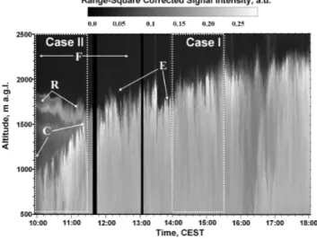
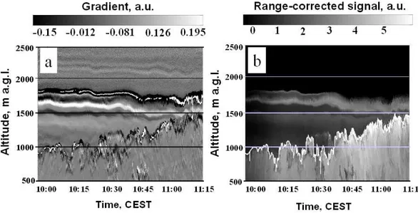
Fig. 2. Time-height cross-section of the range-square-corrected backscatter signal measured on 26 June 2004 from 09:55 to 18:10 CEST. Dotted boxes are the selected regions of Case I and Case II. Temporal and spatial resolutions are 0.033 s and 3 m, re-spectively. R: a strong residual layer from previous day showed up around 1.8 km a.g.l., F: free atmospheric air with very low aerosol load above 2.0 km a.g.l., C: CBL growth during morning eroded the nighttime stable residual layer, E: entrainment at the top of the CBL. Black stripes mark two gaps where no data are available.
UHOH lidar system collected data up to 12 km above ground level (a.g.l.). Figure 2 depicts the time-height cross-section of an eight hour observation of the background-subtracted and range-square-corrected signal in the 1064-nm channel collected between 09:55 and 18:00 CEST on 26 June 2004.
The data is plotted with the maximum resolution possible by the present system, i.e., a time resolution of 0.033 s and a vertical resolution of 3 m. Small-scale turbulent activity in the CBL is clearly visible. This figure demonstrates the UHOH lidar’s capability to observe the boundary layer with ultra-high resolution and to provide a detailed view on fine structures of the aerosol distributions.
The time-height cross-section shows that a previous night RL marked by “R” was present at altitudes between 1.6 and 1.7 km in the morning until 11:20 CEST while the free-tropospheric air with very low aerosol load was present above 2.1 km altitude (marked by “F”). The RL is the previous day’s mixed layer that the new CBL grows into, and as such lies immediately above the CBL. There is also a very thin AL above the RL at an altitude of 1.8 km (see Fig. 2, a separate, third layer above the RL). Around 11:30 CEST, the growing CBL (marked by “C”) reached the level of the RL merging with it so that both became indistinguishable. Such over-shoots are considered to be caused by the initial development of large convective rolls, which turn into more random mo-tions after the quasi-steady equilibrium. Also visible is that starting at 11:20 CEST, the dust layer became trapped in the entrainment region (marked by “E”). This is called
penetra-tive convection (Deardorff et al., 1969). As a result of this ac-tivity, cleaner air from the FT enters the CBL by downdrafts. The RL at 1.6 km a.g.l. in the present case was also observed in the lidar data collected on the previous night (not shown here). Influenced by this process, the CBL grew in thickness and thus a one-way entrainment dominated. When laminar air from the FT and capping inversion are introduced into the CBL, the thickness of the CBL grows. On the contrary, none of the turbulent air is incorporated into the laminar air of the FT. These characteristics were clearly observed by the UHOH lidar measurements.
Between 12:00 and 18:00 CEST, the height of the CBL re-mained nearly constant around 2.0 km a.g.l. In summary, we found two different regimes of the CBL evolution: one dur-ing the rapid growth of the CBL until 12:00 CEST and one in the afternoon with equilibrium entrainment i.e., when CBL evolution is in a quasi-steady state. The quasi-stationary CBL (referred to as Case I in the following) is used first to demonstrate the three techniques for CBL height as well as higher-order moments determination. These analyses were then extended to study the CBL in the morning (Case II). 5.1 Case I: Quasi-stationary convective boundary layer
5.1.1 Results obtained with logarithm gradient method, inflection point method, and Haar wavelet trans-form analysis
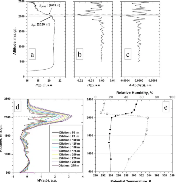
Figure 3 illustrates the retrieval ofzLGM,zIP, andzHWTfor backscatter signals acquired at 15:52 CEST on 26 June 2004. Before the LGM, IP, and HWT were applied to the lidar data, 10 consecutive lidar profiles were averaged which provided a time resolution of 0.33 s.
In the following analysis for LGM and IP method, no fur-ther time averaging was performed. Instead, a gliding av-erage with a Gaussian window of full width at half maxi-mum of 30 m was applied in height to the stored lidar profiles beforeD(z)was calculated. This averaging was necessary to determine the minimum gradient peak. The influence of changing height difference (dz=z2−z1)onD(z)was tested. After performing this sensitivity test, the appropriate peak in theD(z)profile related to the ABL top was found. For these data, dzof 30 m was found to be most appropriate for search-ing the minimum ofD(z).
Fig. 3. Determination of the instantaneous height of the CBL on 26 June 2004 at 15:52 CEST using LGM, IP method, and HWT-based approach. (a)the background-subtracted range-square corrected backscatter signal,(b) the 1st derivative of its logarithm, (c)the 2nd derivative. The temporal and spatial resolution of the data is 0.33 s and 3 m, respectively. In height, a 30 m gliding average is applied.zLGM andzIPare found at 2063 m and 2020 m a.g.l., respectively. (d)Wavelet covariance transformWf(a,b)values for different dilations from
50 m to 275 m. For dilations greater than 175 m,Wf(a,b)shows a clear maximum at 2030 m.(e)Profiles of the potential temperature (bold
dots with solid line) and relative humidity (dashed line) obtained from the radiosonde launch at 14:00 CEST from Schnarrenberg, Stuttgart (48.8333◦N, 9.2000◦E, 315 m a.s.l.) on 26 June 2004.
implieszLGM> zIP(Figs. 3 and 4). Depending upon the tur-bulent activity present in the CBL, the local discontinuity be-tween CBL and FT atop is defined as the transition zone here. This transition zone is also a means of determining the EZT in different atmospheric conditions (Sect. 4.2).
The HWT-based analysis was applied to the same data to determine the CBL height. The wavelet covariance trans-formWf(a,b)was computed for each profile and the
alti-tude corresponding to its maximum was denoted as the CBL top. The crucial point for estimating CBL height following this approach is dependent on the choice of two parameters:
the interval between upper (zmax)and lower (zmin)altitude where the HWT should be applied, and the values of the di-lationa and translationb. Following Davis et al. (2000), a sensitivity test was performed to obtain the characteristic dif-ferences ofWf(a,b)for different dilations as shown in Fig. 3
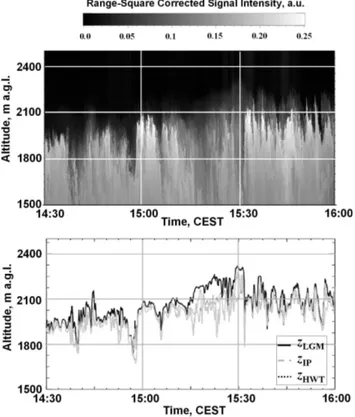
Fig. 4. Zoom-in-view of the time-height cross-section of range-square corrected signal during Case I (upper panel) and the time series ofzLGM,zHWT, andzIP(lower panel).
otherwise stated, the HWT analysis was constrained between the heights of 500 and 3000 m a.g.l.
The HWT coefficient becomes maximal when the covari-ance between backscatter profile and the Haar function is maximum. Brooks (2003) showed how the HWT method identifies a point close to the center of the transition zone, with a trend towards higher values with increasing dilation. Thus, HWT method will tend to identify a point lower than the LGM, though the difference will vary both from profile to profile and with dilation for any given profile. This issue is further extended in the next section.
5.1.2 Intercomparison between the different techniques
Figure 4 presents the time-height cross-section of the range-square corrected signal intensity (upper panel) collected be-tween 14:30 and 16:00 CEST and the temporal evolution of zLGM,zIP, andzHWT(lower panel). The two time series us-ing the LGM and the HWT are highly correlated and the lin-ear trends in both cases are very similar. Correlation analy-ses among the three time series were performed. The result-ing correlation coefficients between time series ofzLGMand zHWT,zLGMandzIP, andzIPandzHWTare 0.851, 0.811, and 0.781, respectively. In general,zHWTis lower thanzLGM.
It is important to mention here that the LGM and the HWT analysis become the same as soon as a dilation equal to the
range resolution (in this case 3 m) is applied in the HWT analysis. The HWT method allows limiting the analysis to a chosen range of scales, so that small scale gradients (e.g., caused by noise) do not appear. The HWT coefficient is cal-culated at each height level; caused by this implicit smooth-ing, the technique does not require additional averaging of the signals in height as in the case of the LGM.
Comparison of the mean CBL heights determined from the respective time series yielded a difference of 59 m be-tween the LGM and the HWT-based analysis while a differ-ence of 63 m was found between LGM and IP method. A difference of only 4 m was found when comparing the mean CBL heights estimated by the HWT and IP method.
It is further important to note that the CBL height deter-mined by HWT is in better agreement with the results of the variance profiles (see Sect. 5.5) than the other two tech-niques. Also the “snapshot” view provided by the radiosonde launch at 12:00 UTC on this day from the near-by weather station (Schnarrenberg, Stuttgart) confirmed this fact. We estimate the top of the CBL by calculating the first deriva-tive of the potential temperature (dθ/dz, whereθ is the po-tential temperature) obtained from the radiosonde. The ra-diosonde measurements revealed a strong signature of the temperature inversion and a sharp drop in the RH at an al-titude of 2005 m a.g.l. confirming the mean CBL height of zHWT=2008 m (panel e in Fig. 3). In contrast to this, the LGM-based results do not show such close similarity nei-ther with the variance profile nor with the radiosonde-derived CBL height.
Fig. 5.Retrieval ofzHWTin the presence of several aerosol layers in the CBL during Case II. The HWT has been applied in the altitude range of 500 m to 3000 m with a dilation value of 260 m.(a)time-altitude-plot ofD(z). A broken white line marks the location of the maximum ofWf(a,b).The HWT-based method mostly identifies erroneously the residual aerosol layer height as ABL top in this case.(b)HWT is
applied in selected altitudes. The upper limit has been restricted to below the residual aerosol layer. Time series of CBL topzHWT(white solid line) superimposed on the range-square corrected lidar backscatter intensity. The convectively growing ABL top is identified correctly and is consistent with a strong gradient in the entrainment zone.
of wavelet coefficient. A sloped aerosol backscatter arises due to the changes in aerosol microphysical properties or aerosol concentrations. This is an important source of bias with the wavelet method. Most probably, a difference of around 100 m between the zLGM and zHWT are observed around 15:15 CEST for this reason (Fig. 4, lower panel). A large transition zone during this period can also be seen in the time-height cross-section.
The IP method uses the results from LGM and a number of criteria have to be fulfilled to obtainzIP as a correct es-timate of CBL height (see Sicard et al., 2006, for a detailed discussion on these criteria).
In summary, it can be stated thatzLGMtends to fall within the upper part of the transition zone,zHWTclose to the mid-dle, andzIPnear the bottom (zLGM> zHWT> zIP). We con-ceive that this is a characteristic difference among the tech-niques. It is important to note that for the first time we have compared three different algorithms to find the CBL height from a very high-resolution lidar measurements: 8 h of obser-vation were used for this purpose. Similar differences among the techniques were found for the rest of the time series al-though not shown here.
Furthermore, it is important to note that the inversion which defines the top of the boundary layer is a thermo-dynamic feature. Lidar backscatter is assumed to reflect the thermodynamic inversion closely because it is approx-imately proportional to the aerosol concentration, which is generally well mixed within the CBL, much lower in con-centration in the FT, and thus has a transition that closely
matches the inversion. Aerosol size, however, is a function of humidity, which often falls dramatically across the inver-sion layer. Therefore, the lidar backscatter is thus not truly conserved and differences between the transition zone lim-its of lidar backscatter profile and thermodynamic inversion might exist, at least for some conditions. However, it can be concluded that the HWT-based approach is the most suit-able and prefersuit-able technique for the determination of the in-stantaneous CBL height; limitations certainly exist as some subjective approach has to be applied for lidar data collected during complex situations (as will be shown in the very next section).
5.2 Case II: Convective boundary layer height during its rapid growth in the morning
This section deals with the investigation of CBL evolution between 09:55 and 11:15 CEST on the same day. During this time, the CBL transformed from a stratified structure in the morning to a well-mixed CBL toward noon.
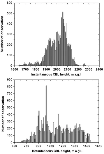
Fig. 6.Frequency distribution of the instantaneous CBL height de-rived by the HWT-based method for Case I (top) and Case II (bot-tom).
A similar analysis was performed for the choice of dilation value as in Case I. A dilation value of 260 m was found suit-able for this dataset. It was mentioned earlier that the value of most suitable dilation depends on the nature of backscat-ter profile. Figure 5a displays that HWT most of the times picked the top of the RL and sometimes AL instead of the top of the convectively growing boundary layer.
The HWT analysis was modified with the following proce-dure. At first, the aerosol layer was identified from the time-versus-altitude plot ofD(z)as displayed in Fig. 5a. Then the upper altitude limit below the aerosol layer was selected and used aszmax(in Eq. 7). The upper limit in the integration for obtaining theWf(a,b)is now not constant but varies in
time. Following this subjective approach (Senff et al., 2002), difficulties arising due to the appearance of RL and AL were eliminated. Figure 5b shows the growth of CBL top (white solid line) overlaid on the range-square-corrected backscat-ter intensity afbackscat-ter the subjective approach was applied. The morning time convection is seen clearly in both figures with the growing CBL top from 0.7 to 1.5 km.
5.3 Entrainment zone thickness for two cases
Two different approaches were studied for estimating the EZT from the time series ofzHWT. First, the standard devia-tion ofzHWTis used (e.g., Davis et al., 1997). This technique assigned here as the standard deviation technique provided an estimate of the mean EZT: 92 m and 185 m for Case I and Case II, respectively. The frequency distributions ofzHWT for both cases are shown in Fig. 6. For Case I (upper panel), the distribution is slightly asymmetric around 2050 m a.g.l. and does not spread much. Larger values are considered to be due to the most energetic thermals. The values around 1700 m a.g.l. were arising mostly during a strong entrain-ment of free-tropospheric clean air. On the other hand, for Case II, the frequency distribution is highly asymmetrical re-flecting an entirely different regime of the CBL (lower panel of Fig. 6). The broader distribution is due to the fact that zHWTis increasing from 900 m to 1500 m in Case II.
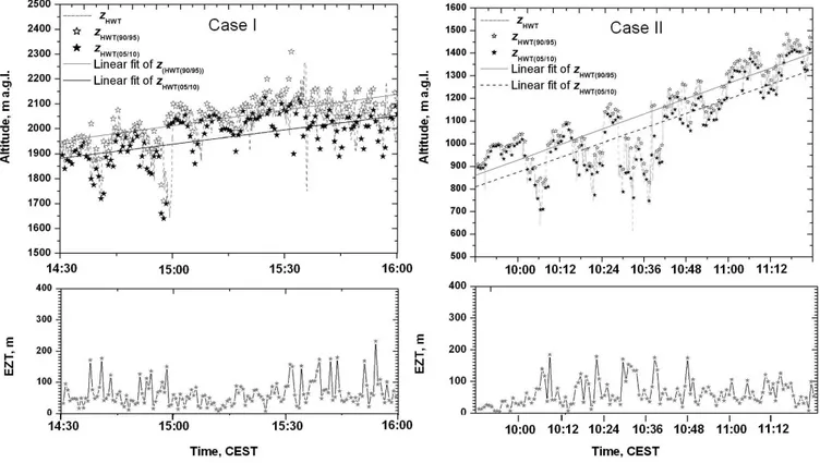
Results obtained with the cumulative frequency distribu-tion method are shown in Fig. 7. This figure shows the evolu-tion ofzHWTwith an illustration of the technique on the time series for both cases. Lower and upper parts of the EZ are denoted aszHWT(05/10)andzHWT(90/95), respectively, where
the first one corresponds to the location of the mean of the 5–10% values of the cumulative frequency distribution and the second one corresponds to the mean of 90–95% values. The difference of these values gives an estimate of the EZT (Fig. 7). 30 s was the averaging time over which the EZT was calculated. The values of EZT for Case I are ranging from about 10 to 230 m (lower left panel) while the mean value of EZT derived by this technique is 75 m. Some higher values of EZT around 200 m might arise due to enhanced convective activity and associated entrainment of the FT air. This mean value of the EZT is approximately 20% smaller compared to the one obtained with the standard deviation method. High values of EZT (up to∼200 m) appear to be correlated with entrainment events of lower FT air.
Results obtained from the cumulative frequency distri-bution method for Case II show the estimated EZT values at each 30 s interval (upper right and lower right panel in Fig. 7). This technique yielded a mean EZT of 62 m while the maximum value of the EZT was 200 m. These types of high resolution measurements of the EZT can be used for experimental validation of the model formulated by Chemel and Staquet (2007) for a CBL.
Fig. 7.EZT determined with cumulative frequency distribution of instantaneous CBL height (zHWT)for Case I (left panel) and Case II (right panel) derived from 0.33 s resolution lidar data. Linear fits for bothzHWT(05/10)(black-dashed line) andzHWT(90/95)(gray-dashed line) of
the cumulative frequency distributions are also shown. The lower panels show the EZT for both cases.
research. Nevertheless, this regime (Case II) has rarely been considered in previous studies of the CBL entrainment zone characterization though being an important aspect with re-spect to near-surface air pollution.
5.4 Evolution of convective boundary layer height
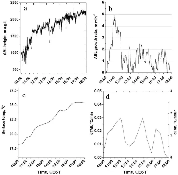
Two different regimes of the CBL growth were clearly observed from the full-day time series of the lidar mea-surements, with respect to the estimated growth rate: one regime (from 09:55 to 11:15 CEST) with growth rate of 4– 5 m/min and another (11:30 to 18:00 CEST) with compar-atively slower rate with 0.5–2 m/min (Fig. 8). This figure shows the time series of CBL height growth rate in m/min (panel b) determined from the time series of thezHWT esti-mated during 10:00–18:00 CEST (panel a). Evolution of the surface temperature (panel c) and rate of temperature change (with respect to timedT/dt, panel d) during the same period are also shown. Growth of the CBL height was highly corre-lated with temperature increase at the surface. Rapid growth in the morning was caused by surface heating and associ-ated convective activities while the decrease of the growth rate and then the persistence of a constant slower growth were most probably due to interaction with the RL and re-sulting capping. The difference in CBL growth rates can be
explained by the surface heat flux behavior. However, de-tails can depend on subsidence, atmospheric stability, etc., but a discussion of these effects on CBL growth rate is be-yond the scope of the paper. The CBL height reached its maximum (2250 m) around 17:30 CEST. This suggests that the surface forcing was still present around this time. Sunset was at 21:30 CEST on this day.
It should be noted that the encroachment at the top of the CBL mentioned in Sect. 5 might be a result of the high correlation between the surface temperature and the CBL height measured during this time. Surface temperature ob-served during 10:00 and 11:30 CEST showed a sharp in-crease from 18.2◦C to 20.2◦C while the CBL height
Fig. 8.The evolution of(a)the CBL height and(b)associated growth rate together with(c)surface temperature and(d)rate of temperature increase between 09:55 and 18:00 CEST on 26 June 2004. Two distinct regimes of CBL growth are found: one with 3–5 m/min and another with 0.5 to 2 m/min. The time series of CBL height and surface temperature between 10:00 and 11:30 CEST show a correlation coefficient of 0.95 indicating that surface heating is responsible for the CBL evolution in this period.
5.5 Vertical profiles of higher-order moments
So far, only the evolution of the CBL top has been dis-cussed. To add further quantitative information, we deter-mine the higher-order moments of particle backscatter coef-ficient fluctuationsβ′
par at different heights to study turbu-lence processes during both cases. Higher order statistics are derived up to an altitude of 2.7 km as it was found pre-viously for these data sets that the CBL height was below 2.7 km a.g.l. We have shown the lower altitude for the ver-tical profiles of integral scale, variance, skewness, and kur-tosis, to be 400 m a.g.l. Below this height, lidar data were affected by partial overlap of the transmitter-receiver geom-etry; one cannot use lidar data collected below these heights without further correction. It should be noted that in addition
to the normalized heightz/ziscale (zi, mean CBL height) in
the profiles of the higher order moments, we also kept the corresponding height in the figures.
5.5.1 Variance spectra
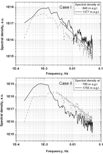
Figure 9 shows the variance spectra of relative particle backscatter coefficient for both observation periods at two different heights. Lidar data with time resolution of 10 s are used here since the errors due to instrument noise would have been unacceptably large at 0.33 s resolution for the purpose of higher-order moments estimation.
lnSF(f )is plotted here against ln(f )whereSF is the
Fig. 9. Spectra of relative particle backscatter coefficient at two different heights for Case I (top) and Case II (bottom). The expected
−5/3-slope of the inertial subrange is shown in each panel.
to the −5/3-power law describing the inertial subrange of the spectra (Kolmogorov, 1941). Obviously, the inertial sub-range was reached in all cases. This confirms that the time resolution used here is high enough to resolve the energy containing eddies and part of the inertial subrange. Engel-mann et al. (2008) showed similar characteristics in the vari-ance spectra ofβpar′ for a case of well-mixed CBL confirm-ingf−5/3roll-off in the spectra. The range resolution of the UHOH lidar (3 m) is higher than for their lidar (75 m) system. Variance spectra of relative particle backscatter coefficient fluctuations at two selected heights for Case II suggest that the inertial subrange was achieved here at the lower height while there is considerable deviation in the higher altitudes as can be seen from the spectra at 1755 m a.g.l.
5.5.2 Autocovariance
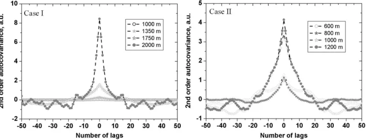
The second-order autocovariance function for each height level was calculated to determine the variance of the particle
backscatter and the corresponding noise variance. The auto-covariance function calculated for 100 lags for four selected heights (1000, 1350, 1750, 2000 m for Case I and 600, 800, 1000, 1200 m for Case II) in the CBL are shown in Fig. 10. The increase of the total variance for zero lag (at 2000 m for Case I and 1200 m for Case II) was due to both the increase of the atmospheric variance and the noise variance. The at-mospheric variance increased sharply because this altitude lies within the EZ.
5.5.3 Integral time scale
The integral time scale can be considered to be the temporal analogy to the integral length scale which is an average dis-tance that energy and mass in the atmosphere can be trans-ported down wind by large coherent eddies present. It is con-sidered to be a useful parameter for numerical modeling of the turbulence and associated trace gas transport in the CBL. In turbulence measurements, a prerequisite for the resolu-tion of the major part of turbulent fluctuaresolu-tions is that integral time scale≫dt where dt is the temporal resolution of the time series. If this condition is achieved, the major part of the horizontal variability of the turbulent eddies is sampled with acceptable resolution so that the inertial subrange in the spectrum and/or the dissipation range in the autocorrelation function becomes resolved. Simultaneously, the vertical res-olution of the measurements must be smaller than the vertical coherence of the turbulent eddies. The high range resolution (3 m) in the UHOH lidar data helped to resolve vertical struc-tures of turbulent fluctuations as will be shown here.
Following Lenschow et al. (2000), we have demonstrated the techniques for reasonable determination of the auto-covariance functions extrapolated-to-zero-lag (described as m11(→0)in their study). In our work the extrapolation for this purpose is performed using the autocovariance function at lag one; we refer to this as 1st lag approach. Figure 11 shows the vertical distribution of the integral scale with and without noise correction for both cases. The profiles of in-tegral scale and higher-order moments were normalized with the mean CBL heightziof 2008 m and 1136 m for Case I and
Case II, respectively. They were estimated by averaging the time series ofzHWTof those periods. These profiles clearly show that without noise correction the integral scale would be significantly underestimated. The standard error due to instrument noise is also shown.
The integral scale for Case I is mostly around 75 s inside the CBL but above 0.8zi this value decreases with height
and attains 35 s nearzi. As shown in Fig. 11 for Case I, the
integral scale values are lying between 40 and 90 s within the normalized height range of 0.2zi and 0.9zi. An increase up
to∼130 s was observed at 1.1zi, which might be explained
Fig. 10.Second-order autocovariance functions for four different heights for Case I (left) and Case II (right). The inertial range is resolved by only 5–7 data points. One lag corresponds to a shift of 10 s of the time series in the autocovariance function.
Fig. 11.The integral scale of particle backscatter coefficient fluctuations determined with and without noise correction for Case I (left) and Case II (right). The vertical coordinate is normalized with the mean boundary layer depth, i.e., the ratio of the heightzand the mean CBL depthzi of 2008 m and 1136 m for Case I and Case II, respectively. The error bars on the profile obtained with 1st lag approach denote the
standard error due to instrument noise.
subrange. Therefore, the major part of turbulent fluctuations in the CBL can be resolved with the UHOH lidar data. This is the key feature of the high-time-resolution elastic lidar system of UHOH as it can be deployed to make turbulence statistics in the CBL. This is quite clear from the figure that a substantial decrease of integral scale is observed from 0.9zi
to the top of the CBL. Couvreux et al. (2005) observed simi-lar decrease of integral scale of moisture due to the presence
of dry tongue in the EZ while Kiemle et al. (1997) observed a slight decrease of the integral scale towards the top of the CBL.
Fig. 12.Vertical distributions of the variance for Case I (left) and Case II (right) with noise correction (1st lag approach) and without any correction. The vertical coordinates are scaled as in Fig. 11. Statistical and sampling errors are plotted with the corrected profiles. A profile ofσβ/βis shown for comparison (solid gray line).
scale value at 1.4zi, can be seen. Above 1.1zi, an increasing
trend was observed up to a high value of about 225 s from 1.5zi to 1.6zi. However, it should be noted that the
turbu-lence scales in the RL are likely much smaller than in the CBL. Consequently, 10 s time resolution used may not be ap-propriate to capture turbulence on the smaller scales. There-fore, it is more challenging to discuss in detail the integral scale in the region of the RL and an embedded thin AL with this technique. Furthermore, lidar measurements showed sig-natures of some organized wave activity associated with the RL. Consequently, the concept of random statistical atmo-spheric fluctuations may not be applicable here.
5.5.4 Variance
Vertical profiles of the variance with and without noise cor-rections for both cases are shown in Fig. 12. This figure shows that noise correction is only necessary between 0.8 and 1.1zi. Variance profiles yielded the variability of the
particle backscatter signal at different height above the li-dar site for both periods. The profile for Case I shows that the variance of the aerosol distribution is approximately con-stant up to 0.8zi (∼1600 m a.g.l.) since the vertical gradient
of the aerosol concentration (D(z)calculated for the entire period, not shown here) in this region are not large enough and nearly constant. The meanD(z)profile confirmed that aerosol particles are uniformly distributed within this heights
implying that a well-mixed CBL regime prevailed. Above this height, variance increases reaching a well-defined max-imum at 2022 m a.g.l. near the CBL top which is related to the large variation of aerosol concentration in the EZ due to rapid mixing of the air parcels between the CBL and the FT (Deardorff, 1972).
In a well-mixed CBL regime, very often sharp gradients in aerosol concentration exist through the EZ at the CBL top as cleaner from the FT is entrained and mixed into the aerosol-laden CBL. Since this variance profile (averaged over 1.5-h) can be considered as a space-averaged profile, the fluctua-tions of the inversion layer do not affect to the location of the maximum of the variance but make it more spread. This height can be considered as the mean CBL height over this time period indicating the location of most of the exchange processes between the CBL and the FT. These properties of the variance profile ofβpar′ are similar to the findings of Wulfmeyer (1999b) concerning the humidity variance, how-ever, the shape near maximum is much sharper in the EZ in our case.
In contrast to theV profile of Case I, for Case II, there is a very broad peak between 700 m (∼0.6zi)and 1000 m
(0.9zi), with a local maximum at a little above 910 m in
to 11:15 CEST, with a period of more rapid growth between them (Fig. 5) and also likely due to the non-stationarities present in the CBL height evolution. However, the influence of the different aerosol layers cannot be ignored while ex-plaining the vertical distribution of the variance in this case. Most probably, above 1.2zi, high values ofV corresponded
to the RL and the AL at those heights. The rest of the large variance values were observed due to turbulent activ-ities present in the CBL. Above the RL, the variance profile decreased and reached nearly a value of zero. Further investi-gation of these characteristics needs detailed information on flux Richardson number (Sorbjan, 1990).
It should be noted that the dependence of the particle backscatter coefficient on RH is strongly related to the mi-crophysical properties of the aerosol particles, particularly its hygroscopicity. Wulfmeyer and Feingold (2000) showed the relationship of the aerosol particle backscatter and humid-ity within the boundary layer based on state-of-the-art differ-ential absorption lidar measurements of water vapor. Addi-tionally, they compared their findings with an aerosol model based on the formulation introduced by Fitzgerald (1975) and H¨anel (1976). Randriamiarisoa et al. (2006) showed that RH effect on aerosol microphysical properties is more compli-cated; for instance, hysteresis effects can cause backscatter lidar fluctuations. In Wulfmeyer and Feingold (2000), in the 70–80% RH region, the change ofβpar was about 10%, in Gibert et al. (2007) it was between 10 and 20%, and in Ran-driamiarisoa et al. (2006) it was much larger in some cases, probably due to aerosol components particularly sensitive to RH. In our case, we are convinced that the site was mainly affected by urban aerosol particles so that based on the re-sults of Wulfmeyer and Feingold (2000), the sensitivity in the 70–80% region should be in the order of 10%.
An important issue is the estimation of the variability of RH in the EZ. Unfortunately, only one radiosounding is available, which does not capture this variability. It showed the RH to be up to 70% within and above the CBL (Fig. 3). However, we are able to estimate this variability based on reasonable assumptions concerning boundary layer turbu-lence. Assuming reasonable summertime surface sensible and latent heat fluxes of 200 W m−2, respectively, and a ver-tical convective velocity scale ofw∗≈1 m s−1, we get a
tur-bulent humidity scale of 0.08 g m−3, and a turbulent temper-ature scale ofT∗≈0.16 K. Propagation of this variability in
RH, e.g., using the Magnus equation, we estimate a variabil-ity of RH at the top of the CBL of about 5%. This trans-lates in a variability ofβparof approximately 5% based on the results of Wulfmeyer and Feingold (2000). We have ana-lyzed the profile ofσP/P≈σβ/β, whereσβis the square-root
of variance andβ is the mean profile of particle backscat-ter during the entire measurement period (Fig. 12). This profile shows the normalized variance (in %) of the particle backscatter fluctuation which considers only aerosol contri-bution to lidar backscatter signal. It shows that the variabil-ity ofσβ/β is about 40% in the EZ whereas we determined
a contribution of RH variability of just 5%. Consequently, we can state that the main variability ofσβ/β is determined
by turbulence and not by RH fluctuations. Nevertheless, the analysis performed in this study illustrates the difficulties, but also the possibilities, of detailed analysis of aerosol lidar measurements for studying turbulence characteristics within a CBL.
5.5.5 Skewness
The turbulence structures throughout the entire CBL and above for both cases were further characterized by evaluat-ing the vertical profiles of the skewness. Figure 13 shows the skewness profiles without and with noise correction using a three-point linear extrapolation to zero lag for both cases. Noise error and the sampling error are plotted as error bars on the corrected curve. Vertical structure of the skewness profile shows the presence of significant differences inside the CBL. The estimated noise error is small, but the sampling error is relatively high above the CBL top.
Skewness (third moment) is a measure of the lack of sym-metry of a distribution. For Case I, within the lower half of CBL, we mostly observed skewness values close to zero (nearly Gaussian distribution) with exception of negative val-ues in the regions near 0.4zi. This indicates that the aerosol
particles are evenly distributed (or well mixed) up to 0.5zi.
Within the upper half (i.e., between 0.5 and 0.9zi) of the
CBL, we observed negative skewness. Presence of these neg-ative skewness values in these heights indicates very deep entrainment of clean FT air into the CBL and consequent mixing. The clean FT air gradually mixes with the aerosol particles inside the CBL and mixes out somewhere near the middle of the CBL and reflects highly negative perturba-tions. These observations are strikingly similar to the mois-ture skewness profile during the penetration of dry air pock-ets into the CBL as shown in Couvreux et al. (2005). Near the top of the CBL, a positive prominent peak is observed with Skvalue of about 2. This is likely associated with the center
of the aerosol plumes that are penetrating to this height. For Case II, the skewness profile showed a high variability even inside the CBL with positive values. Predominant nega-tive skewness values up to the height of 0.7ziwere the result
of rapid growth of the CBL height during Case II. Similar results were found by Mahrt (1991), Couvreux et al. (2007), and Larson et al. (2001). For instance, Couvreux et al. (2007) clearly mentioned in their study: “The rapid CBL growth ex-plains why greater negative skewness is observed during the growing phase. . . ”. It should be noted that negative skewness is observed up to∼800 m a.g.l. This perhaps underlines the importance of entrainment processes down to very low alti-tudes during the rapid growth of CBL.
Above 800 m, positive skewness was found. It is interest-ing to note that theSk profile increased with height in two
different altitude regimes: one from 0.8zi and 1.1zi and
Fig. 13.Same as Fig. 11 but for skewnessSkfor Case I (left) and Case II (right). For a Gaussian distribution,Skis 0 (gray solid-lines).
is representative for convective activity, which organized as height increased but the second one exhibited several peaks, which were arising most probably due to the presence of dif-ferent scales of mixing. Above an altitude of 1.5zi, theSk
profile obtained a constant value close to−1 due to almost homogeneous aerosol distributions in the FT. It might be the case that the AL at 1.8 km has different turbulence charac-teristics than the RL; however, we can not accurately differ-entiate and quantify the differences between the AL and RL with the present data set. It should be noted that comparisons of these results with similarity relationships and scaling with standard turbulent scales in the CBL must be avoided. 5.5.6 Kurtosis
Figure 14 presents the kurtosis profile with and without noise correction for both cases. The sampling and noise errors are shown on the corrected kurtosis profile. First lag and linear fit approach provide here nearly identical results, so we kept the one corresponding to the first lag approach.
Kurtosis (fourth moment), a measure of the flatness of a distribution indicating whether the data distribution is nar-row or flat relative to a normal distribution, is considered to be another important parameter in turbulence studies. In the present context, the value of kurtosis is expected to provide an indication of the degree of mixing at different heights.
Figure 14 shows a constant value ofK around 3 corre-sponding to a nearly-Gaussian shape of the distribution of βpar′ (for Case I) up to an altitude of 0.6zi. However, between
0.6 and 0.9ziit shows a small increase ofKbetween 4 and 5
which indicates that the distribution is more peaked here.K increases to 12 (four times larger than those of a pure Gaus-sian distribution) just above the top of the CBL which ex-plains that the distribution has a more acute peak (around the mean) here than that within the CBL which might be arising due to the vigorous mixing at the regions of active entrain-ment dynamics. This agrees with the findings of Lenschow et al. (2000). A high value ofKindicates that the most vari-ability is due to the presence of infrequent extreme deviations in the time series ofβ′
parat those heights. On the other hand, a low value ofK signifies a time series with most measure-ments clustered around the mean yielding a well-mixed CBL regime . For Case II, the kurtosis increased with height by a factor of∼2.5 in the region of CBL height.
5.6 Comparison of Case I and Case II
The key difference in the characteristics of the two cases is due to two main reasons. Firstly, a rapid growth of CBL height prevailed during Case II while for Case I, a very slow growth was found which could be considered as a quasi-stationary CBL. Secondly, unlike Case II, no strong RL or any detached multiple aerosol layers were observed during Case I. Similar behaviors were observed for both cases while demonstrating the CBL height estimation with LGM, IP method and the HWT-based analysis, i.e., the fundamental difference among the techniques providingzLGM> zHWT> zIP.
Fig. 14.Same as Fig. 11 but for kurtosisKfor Case I (left) and Case II (right). A Gaussian distribution showsK=3 (vertical solid lines on both panels).
Fig. 15.FFT power spectra of the time series ofzHWTobtained for Case I (gray line) and Case II (black solid line). The−5/3 power law curve is shown for comparison. A spectral exponent value of 1.00±0.06 and 1.50±0.04 are found for Case I and Case II, respec-tively.
based on the time series analysis (e.g. Pelletier, 1997; Boers et al., 1995) have shown that the power-law dependence can be found fromSF(f )∼f−γ whereSF is the power, f is
the frequency andγ is the corresponding spectral exponent. The slope of ln[SF(f )] versus ln[f] yields the value ofγ. If
1< γ <3 then, the signal is a non-stationary process with sta-tionary increments. Davis et al. (1994) presented a detailed
discussion on the spectral properties and stationary issues for time series of geophysical datasets. Such FFT-based spectral analysis of the CBL height time series provided spectral ex-ponent values of 1.00±0.06 and 1.50±0.04 for Case I and Case II, respectively (Fig. 15). For Case II, the spectral ex-ponent value was lying in the region 1< γ <3. This is a confirmation of the implicit non-stationarity present during Case II. For Case I, the spectral exponent value confirmed the quasi-stationary CBL regime. Additionally, there are some distortions in the low frequency tail of the spectrum of Case II. They are arising most probably due to the pres-ence of a trend (an increasing one) in the time series pro-ducing non-stationarity in it. The temporal resolution of the analyzed time series is 0.33 s. Therefore, the Nyquist fre-quency (fmax/2) for the FFT spectra is 1.66 Hz. None of the slopes confirm the−5/3-power law dependency. We con-ceive that the difference in the spectral exponent values is due to very different regimes of the convective activities present: the CBL time series, for Case I, this is entirely governed by the mixing in the EZ while for Case II, this is partially influ-enced by the entrainment in the RL atop.
values to be dependent on the dynamic stability conditions in the CBL as well as to be sensitive to the grid resolution of the LES model used. These power law exponent values can be used operationally to separate stationary from non-stationary characteristics of CBL height on the basis of long term datasets. Furthermore, this information is beneficial to find some quantitative aspects of the time series. For in-stance, Perera et al. (1994) found the spectral exponent value to be 2 for intermittent wave breaking events in their mixing box experiments.
A detailed comparison among the vertical distribution of the higher-order moments profiles for both cases were al-ready discussed in the previous section. Furthermore, it should be noted that the results obtained after the higher-order moments analysis are based on the assumption that hy-groscopic growth of the aerosol particles can be neglected. It has been found that such assumptions are not considered to be fully true for the CBL regime during Case II both due to the heterogeneity in the distributions of the aerosol parti-cles influenced by a rapid growth of CBL, and the presence of the RL and the AL above: certain sections of the profiles of higher-order moments thus include a mixture of data from above the CBL, within the active EZ, and within the body of the CBL. The relative fractions of each vary with altitude. Such a blending of data from different turbulent regimes af-fected the proposed interpretations of the profiles. However, it cannot be avoided that smearing takes place in regions with rapid CBL growth. Nevertheless, this kind of meteorological measurements are necessary for a description of the turbu-lence in the CBL regime even during its rapid growth as was shown in Couvreux et al. (2007) explaining the rapid growth to be the source of the negative water vapor skewness in the CBL.
6 Summary and outlook
Within this paper, the benefits of high-resolution measure-ments obtained with a vertically-pointing aerosol lidar for detailed CBL analyses are demonstrated. The data presented here, were collected over an urban region during an 8-h ob-serving period in the daytime. The lidar system has spatial resolution of 3 m and a pulse repetition rate of 30 Hz, and therefore outperforms lidars used previously for such studies of the CBL and the entrainment zone, where high resolution measurements are highly beneficial.
The quasi-continuous vertically-pointing lidar measure-ments showed detailed insights into two different regimes of CBL on a certain day: a quasi-stationary well-mixed cloud free CBL (Case I) and a rapidly growing CBL in the morning in presence of a strong RL over the CBL top (Case II). Three different gradient-based approaches (LGM, IP, and HWT) are compared for precise determination of the instantaneous CBL height. Furthermore, EZT is determined. The HWT-based analysis is found to be the most robust technique.
Ad-ditionally, the HWT-based approach was successful in de-termining the CBL height also in complex situations like in Case II.
The evolution of the instantaneous CBL height through the course of the day is discussed. Two different growth rates are found: a high growth rate of up to 5 m/min in the morning and a relatively lower value of around 1 m/min in the after-noon. The instantaneous CBL heights varied between 0.6 and 2.3 km a.g.l. during the day. The mean EZT in the morn-ing was lower (62 m) than in the afternoon (75 m). These val-ues are obtained with the cumulative frequency distribution method. The spectral exponent value obtained in the energy spectrum for Case II, confirmed the non-stationary behavior. Its value of 1.50±0.04 obtained for Case II is similar to the findings (1.60) of Boers et al. (1995) who investigated the ABL height in a trade-wind cumulus regime. These results can be applied for CBL modeling (Pelletier, 1997).
For the first time, aerosol lidar measurements were used for higher-order moments calculation of the aerosol backscatter field. This gave a comprehensive description of the atmospheric turbulence and aerosol inhomogeneities. This method can be applied for a well-mixed CBL regime if the fluctuations of aerosol microphysical properties can be neglected. It was demonstrated that the major part of the in-ertial subrange was detected and that the measured integral scales were significantly larger than the temporal resolution of the lidar data. Consequently, the major part of turbulent fluctuations was resolved. Power spectrum analysis of the aerosol backscatter fluctuations at various heights inside the CBL showed a roll-off according tof−5/3-power law which suggests that the inertial subrange was reached.