www.atmos-meas-tech.net/5/1965/2012/ doi:10.5194/amt-5-1965-2012
© Author(s) 2012. CC Attribution 3.0 License.
Measurement
Techniques
Lidar measurement of planetary boundary layer height and
comparison with microwave profiling radiometer observation
Z. Wang1,2, X. Cao1, L. Zhang1, J. Notholt2, B. Zhou1, R. Liu1, and B. Zhang1
1Key Laboratory for Semi-Arid Climate Change of the Ministry of Education, College of Atmospheric Sciences, Lanzhou University, Lanzhou, 730000, China
2Institute of Environmental Physics, University of Bremen, 28334 Bremen, Germany
Correspondence to:L. Zhang ([email protected])
Received: 18 January 2012 – Published in Atmos. Meas. Tech. Discuss.: 7 February 2012 Revised: 6 July 2012 – Accepted: 18 July 2012 – Published: 14 August 2012
Abstract. The atmospheric boundary layer height was de-rived at two locations in the city of Lanzhou (China) and its suburb rural area Yuzhong. The aerosol backscatter li-dar measurements were analysed using a wavelet technol-ogy and the parcel method was applied to profiling mi-crowave radiometer observations. For a few occasions the average boundary layer height and entrainment zone thick-ness was derived in convective situations at Yuzhong. Re-sults from selected observation days show that both datasets agree in strong convective situations. However, for weak con-vective situations the lidar measurements reveal boundary layer heights that are higher compared to the microwave observations, because a decrease of the thermal boundary layer height does not directly lead to a change of aerosols in that altitude layer. Finally, the entrainment zone thick-nesses are compared with theoretical predictions, and the results show that the measurements are compatible with theoretical models.
1 Introduction
The boundary layer height (BLH) is a key parameter in describing the structure of the atmospheric boundary layer (BL), it determines the volume available for pollutant disper-sion. Currently, the BLH cannot be measured directly but can be estimated from remote-sensing profile measurements. The lidar remote-sensing instrument is a useful tool to measure properties of the BL and the BLH.
Lidar backscatter profiles represent the vertical distribu-tion of the aerosol concentradistribu-tion in the atmosphere.
Gener-ally, most aerosols have their sources at the surface, produc-ing high concentrations in the BL relative to the free atmo-sphere above. There are usually sharp gradients in aerosol concentration at the BL top, this provides a method to determine the BLH.
the lidar aerosol profile has its strongest negative gradients, however, this position does not always correspond to the BL top. In our approach, instead of just selecting the maximum negative gradient, multiple positions are selected and then the BL top is determined by assuming the continuity in the evolution of BL top as a function of time.
The entrainment zone thickness is another important pa-rameter of the BL. The entrainment zone is located at the top of the BL and consists of a mixture of air from the BL below and free-troposphere characteristics from above. It is defined as the region with negative buoyancy flux (Stull, 1988). However, various alternative definitions occur in mea-surements because of different means (Boers and Eloranta, 1986; Nelson et al., 1989; Flamant et al., 1997; Grabon et al., 2010). In this paper, the definition used by Cohn and Angevi-neet (2000) is applied, whose algorithm searches for the lo-cations of percentiles of the BL top. The results are compared with that from theoretical models.
The following Sect. 2 introduces the sites and measure-ments. The method is described in Sect. 3, results are shown in Sect. 4, and Sect. 5 gives the summary and discussion.
2 Observation sites and instrumentation
The data used in this paper have been recorded at the Semi-Arid Climate Observatory and Laboratory of Lanzhou Uni-versity (SACOL) including two sites located at the suburb rural area of Lanzhou – Yuzhong (SACOL-Main, 35.950◦N, 104.133◦E, 1965.8 m) and the city of Lanzhou
(SACOL-Lanzhou, 36.054◦N, 103.859◦E, 1525.0 m, 48 km far from
SACOL-Main), respectively. All the instruments used are operated at SACOL-Main except for the lidar (CE370-2) at SACOL-Lanzhou.
The micro-pulse lidar (CE370-2) includes a co-axial sys-tem with a 20 cm diameter receiving telescope and a Q-switched frequency doubled Nd: YAG laser operated at 532 nm. The pulse repetition frequency is configured to 4.7 kHz. It is capable of obtaining the aerosol vertical profiles from the ground up to 30 km altitude with an altitude resolu-tion of 15 m. The lidar (MPL-4) uses an Nd:YLF pulsed laser diode, operating at 527 nm. The aerosol and cloud measure-ments are recorded with a spatial resolution of 75 m and at a temporal resolution of 1 min.
The microwave radiometer (TP/WVP-3000) is a passive remote-sensing instrument. It has two systems for measure-ments of the temperature and relative humidity profiles. It works at 22–60 GHz, where the spectral region 22–30 GHz is used for the water vapour profile and the 51–59 GHz region to determine the temperature profile. The radiometer allow obtaining the vertical profiles of temperature, water vapour and liquid water from the ground up to 10 km altitude with a time resolution of 1 min. Below the 1 km height, the altitude resolution is 0.1 km, above 0.25 km.
0 1 2 3 4 5 6
0.0 0.2 0.4 0.6 0.8 1.0 0 1 2 3 4 5 6
-0.08 -0.04 0.00 0.04 0.08
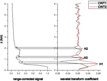
Fig. 1.Illustration for wavelet transformation, CWT1is used to
de-tect the particle layer, and CWT2is used to follow the negative
gra-dients of lidar profile. The minima of CWT1corresponding to the
base and top of particle layer, are indicated by the arrows. The max-ima of CWT2correspond to the positions of negative gradients, and
H1, H2, H3 are the first three maxima.
The fluxes of momentum, latent and sensible heat are mea-sured at 3.0 m altitude with a three-axis sonic anemometer (CSAT3, Campbell) pointing into the prevailing wind di-rection and an opened path infrared CO and HO analyser (LI7500, LI-COR). These signals are logged to a data log-ger (CR5000, Campbell) at 10 Hz.
3 Methodology
3.1 The detection of the BLH
The BLH is determined according to the sharp gradient of lidar profile at the top of the BL, however, the sharp gradient also occurs at the top of clouds or advected aerosols layers which, therefore, should also be identified. The continuous wavelet transform (CWT) for each lidar profile is given by
CWTi(a, b)= z2 Z
z1
p (z, t ) gi
z
−b a
1
√adz, i=1,2 (1)
g1(t )=(1−t2)e−t
2
2.√
2π (2)
g2(t )= −t e−t
2
2.√
2π (3)
0 4 8 12 16 20 24 0.0
0.5 1.0 1.5 2.0 2.5 3.0
0 4 8 12 16 20 24
0 1 2 3 4 5 6 7
z(
k
m
)
t (UTC+8)
H1 H2 H3 28 Jan. 2007
z(
k
m
)
t (UTC+8)
H1 H2 H3 cloud 07 Jan. 2007
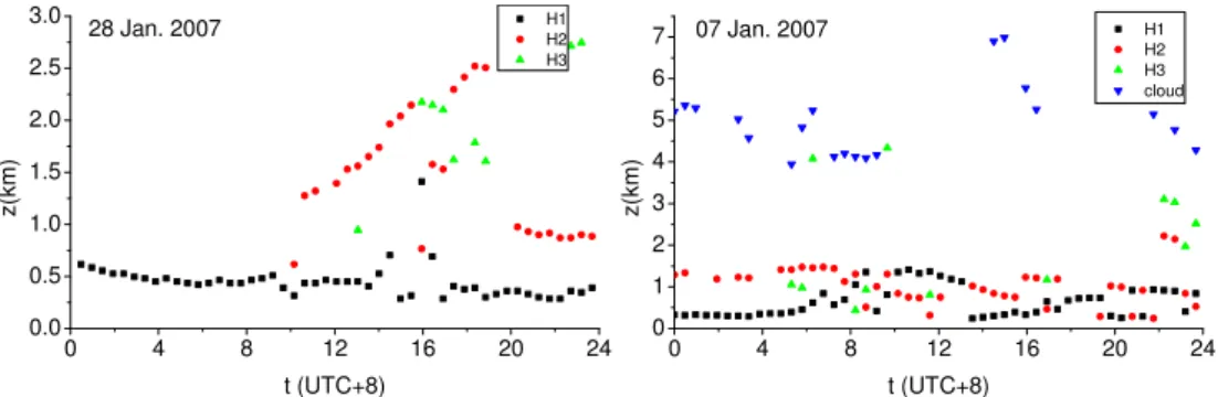
Fig. 2.Temporal evolution of aerosol layer height on two days in January 2007. Each dot represents the average for five minutes measure-ments. Measurements were taken every 30 min.
0 4 8 12 16 20 24
0 1 2 3 4 5 6 7
0 4 8 12 16 20 24
0 1 2 3 4 5 6 7
z(k
m
)
t (UTC+8) BLH
clloud or aerosols layer 10 Jun. 2008
z(k
m
)
t (UTC+8)
BLH cloud 06 Jul. 2008
Fig. 3.The diurnal evolution of BLH on two days during summer of 2008. Each dot represents the average for five minutes measurements. Measurements were taken every 30 min.
considered true. The method of detecting the particle layer is the same as used by Morille et al. (2007). They recom-mend ten times the noise level as threshold value. In our case, a visual estimated value is used to all measurements. Similarly, CWT2(a, b)has its maximum at the part of li-dar profile where the altitucorrected backscatter signal de-creases with height. The working principle of the wavelet transformation is illustrated in Fig. 1. The largest maximum of CWT2(a, b)often occurs at the top of the BL when both cloud and advected aerosols layer are absent. Currently the following method is applied to retrieve the BLH.
– The first, second and third largest values (H1, H2, H3) are selected as maxima of CWT2(a, b)except for those corresponding to cloud and advected aerosol layers top. During cloudy situations, only those maxima located under the base of the cloud are considered. The loca-tions of the three maximums likely denote the BL top.
– “oldblh” is defined as the average of five successive BLHs during a time interval directly before the lidar sig-nal. “oldblh” represents the average of the earlier BLHs and is used to characterise the degree to which the posi-tions of currentH1,H2 andH3 depart from the former BL top.
– After that, the analysis continues in the following way: 1. During cloudfree conditions, assuming that there
is an advected aerosol layer and all maxima of CWT2(a, b) are located below the base of this aerosol layer are smaller than zero then the one closest to oldblh between its top and base will be considered as the BL top.
2. If Eq. (1) does not match, there is a cloud or advected aerosol layer and H1 is smaller than a threshold value “thre2”. In that case the base of this cloud or aerosol layer will be considered as the BL top. Only those maxima of CWT2(a, b) that are larger than this threshold value are considered as corresponding to some features of the boundary structure other than noise fluctuations. In this case there is a cloud or aerosol layer located at the top of the boundary layer (Morille et al., 2007).
3. If Eqs. (1) and (2) do not match, the following func-tions will be applied,
r (x)=min(e−x−σc(t ),1) (4)
ratio=H
H1 (5)
Fig. 4.Comparison between results from lidar and microwave pro-filing radiometer measurements for 29 July 2007. The dotted line represents the BLH from the microwave profiling radiometer de-termined by the parcel method and each dot is the average for five minutes measurements.
c(t )/5 ln 2. The stronger thermal convection is in the BL, where the range, c (t ) is larger. Here, we just assume that c (t )increases linearly before 12:00 of local time and then maintain constant after that.H represents the value between H2 and H3 whose altitude is closer to “oldblh”. A large r (|zH1−oldblh|)means a larger possibility that the altitude ofH1 denotes the true BLH, a large “ratio” means a reverse one. If ratio is larger thanr (|zH1−oldblh|), then the location ofHwill be considered as the BL top, otherwise the location of H1 is accepted. This criterion guarantees the temporal continuity of the development of the BLH. The parameters in the expressions above, vary according to the time resolu-tion of the lidar data; the larger the interval between the two successive records is, the less important it is.
3.2 Average BLH and entrainment zone thickness
The entrainment zone thickness can be calculated from the temporal (Wilde et al., 1985; Cohn et al., 2000) or spatial (Flamant et al., 1997) variation of local BLH top. A sin-gle lidar profile from MPL-4 represents an average for one minute measurements. The BLH from the single profile de-notes the local BLH, so the average BLH and the entrain-ment zone thickness can be derived from temporal develop-ment. The method used here is the same as that proposed by Cohn et al. (2000). First, a cumulative probability distribu-tion (CPD) is calculated from the occurrence of the sequence of the BLH values for 1 h, whose trend has been removed by fitting a second-order polynomial. Second, the value cor-responding to 10 %, 90 % and 50 % of CPD is added to the second-order polynomial to give the base, top of the entrain-ment zone and the average BLH, respectively. The percent-ages defining the top and base of entrainment zone are dif-ferent from those proposed by Wilde et al. (1985) and Cohn et al. (2000). Flamant et al. (1997) proposed an approach to determine these quantities from correlated atmospheric lidar and in situ measurements.
3.3 Parameterisation theory of entrainment zone thickness
According to parcel theory, the entrainment zone thickness is related to the kinetic energy and resistance of the air parcel rising (Bores and Eloranta, 1986). It can be written as:1h∝g1θw2
/θ0, where1h is the entrainment zone
thick-ness,gis the gravitational constant,1θis the potential tem-perature change across the entrainment zone,θ0is the aver-age potential temperature in the BL, andwis the vertical ve-locity.wis typically characterised by the convective velocity scale defined as:w3∗=g(w′θ′)sh
θ0 , wherehis the average BLH
and(w′θ′)s is the kinematic heat flux at the surface.
Gryn-ing and Batchvarova (1994) derived another parameterisa-tion based on the turbulent-kinetic-energy equaparameterisa-tion. It can be written as: 1hh ∝(RiE)−1/3, withRiE=(g/θ0h1θ
w2
e as the
en-trainment Richardson number,we=∂h∂t −wLis the entrain-ment velocity, andwLis the large-scale mean vertical veloc-ity, which can be neglected in case of strong convection. In addition, 1hh ∝we
w∗
α
as proposed by Nelson et al. (1989), where three possible exponents 1.0, 0.5 and 0.25 are sug-gested. The retrieved entrainment zone thickness is examined through those theories, the kinematic heat flux at the surface is provided by the three-axis sonic anemometer, and the mean potential temperature of the BL and the potential temperature change across the entrainment zone are derived from temper-ature profiles by the microwave profiling radiometer. For the BLH, the one given by the lidar-MPL is used. However, there may be relatively large errors in the potential temperature change across the entrainment zone due to the limited verti-cal resolution of the profile data of the profiling radiometer.
4 Results
8 10 12 14 16 18 20 0
1 2 3 4
t (UTC+8) 09 Jun. 2007
z(km)
0.0 0.5 1.0 1.5 2.0 2.5
8 10 12 14 16 18 20 22
z(k
m
)
14 Jul. 2007
t (UTC+8)
10 12 14 16 18 20
0.0 0.5 1.0 1.5 2.0 2.5
z(k
m
)
t (UTC+8) 05 Aug. 2007
8 10 12 14 16 18 20
0.0 0.5 1.0 1.5
17 Sept. 2007
z(
km)
t (UTC+8)
8 10 12 14 16 18 20
0.0 0.2 0.4 0.6 0.8 1.0
22 Nov. 2007
z(k
m
)
t (UTC+8)
8 10 12 14 16 18
0.0 0.2 0.4 0.6 0.8
14 Dec. 2007
z(k
m
)
t (UTC+8)
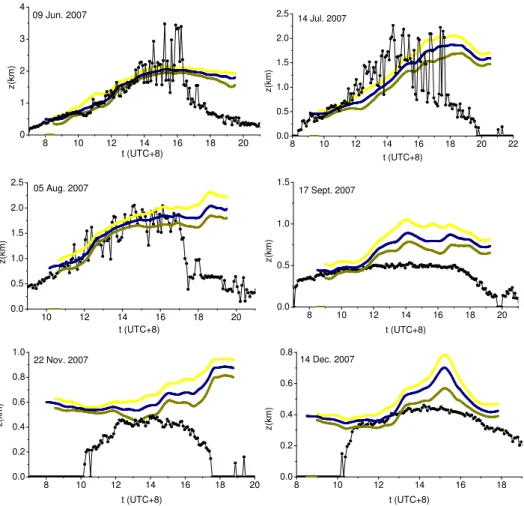
Fig. 5.Comparisons between the BLH from lidar and microwave profiling radiometer for six measurement days in the period of June to December 2007. The contents are the same as Fig. 3, except that temperature measurements are not showed.
result in values for the BLHs which do not necessarily agree with each other. Van Pul (1994) compared the BLH of noon from lidar and radiosondes, and found both agree well. Emeis et al. (2004) compared the BL structures determined by a sodar, by a rass (radio acoustic sounding system) and by a ceilometer. Wiegner et al. (2006) presented a comparison of a comprehensive set of instruments and methodologies. Emeis et al. (2008a) summarised and compared various approaches for determining the BLH from acoustic, optical and electro-magnetic remote sensing. In the following, the BLHaerosol and BLHtempare used to represent the BLH from the aerosol distribution and temperature profile, respectively.
4.1 The BL in the city of Lanzhou
Figures 2 and 3 show four cases of lidar-CE370 under nearly fair weather conditions, performed at SACOL-Lanzhou. Lanzhou is located in a valley basin. The basin is ellipti-cal, surrounded by mountains with the Yellow River flow-ing through the city. The geography and meteorological con-ditions make it difficult for pollutants to diffuse. The verti-cal distributions of aerosols in the BL usually show a
com-plicated multi-layer structure. Figure 1 shows the evolution ofH1,H2 andH3 to illustrate their different features. On 28 January 2007, onlyH2 andH3 when larger than 0.15H1 have been shown, and 0.25H1 on 7 January 2007 (Fig. 2). Figure 3 shows the evolution of the BLHaerosolfor two days in 2008.
On 28 January 2007 (Fig. 2), the aerosol concentrations for the whole day below 0.5 km are relatively high compared to the ones above 0.5 km. There is a very strong gradient in the aerosol concentration at the top of the aerosol layer, and H1 mainly denotes its top. After 09:00, the thermal rising of the air-masses produce a second aerosol layer with a weak gradient at its top above the first one,H2 denotes its top be-fore 16:00. On 10 June 2008 (Fig. 3), from 08:00 to 12:00, there are clouds at 3.0 km altitude initially which dissipated but then appeared again later. The BLHaerosolfor the cloud-free conditions are not correct.
Fig. 6.Comparison of entrainment zone data with theoretical values:(a)entrainment zone thickness, (b)normalised entrainment zone
thickness and entrainment Richardson number,(c)normalised entrainment zone thickness and ratio of entrainment velocity and convective
velocity scale.
al. (2000) might be more suitable. Both of them determine multiple aerosol layers from each lidar profile.
4.2 The BL in suburb rural area of Lanzhou – Yuzhong
Figure 4 shows the results from the lidar-MPL and mi-crowave profiling radiometer measurements on 29 July 2007 at SACOL-Main. Between 11:00 and 16:00 the BLHaerosolis about 0.5 km lower than the BLHtempfrom microwave pro-filing radiometer. The latter begins to rise rapidly from 11:00 on while the result from the lidar increases more slowly. This delay in the development of aerosol distribution compared to the development of the thermal structure of the bound-ary layer has been revealed by Emeis and Schafer (2006) and Emeis et al. (2008b) using sodar and ceilometers. Af-ter 16:00, the BLHtempdecreases quickly and disappears at 20:00, but the results from lidar maintain at 2.0 km altitude. This discrepancy can be assigned to the fact that the BLHtemp represents an upper limit altitude which the rising thermal air-masses can reach while the BLHaerosol, representing the height of the aerosol layer, does not drop immediately as the temperature decreases, since the aerosols concentrations do not dilute when mixing with the surrounding air immediately. Figure 5 shows results for six measurement days between June and December 2007 at SACOL-Main. In situations with
strong convection, the BLHaerosolagrees with BLHtemp, such as the examples in June, July and August show. However, in situations with weak convection, the BLHaerosolis markedly higher, as shown by the observations in September, Novem-ber and DecemNovem-ber. Another feature is the abrupt decline of BLHtempin the afternoon, where the BLHaerosolmaintain its altitude roughly or decreases slowly. The BLHtempis mainly determined by the thermal condition in the BL, it can de-scribe the evolution of the convective BL in the morning when thermal turbulence dominates. The BLHaerosoldoes not always follow this development. BLHaerosolstill denotes the height of aerosol layer formed at night, such as the case of November and December. However, in the afternoon the con-vective BL departs into a residual layer and a stable layer, where the BLHaerosol likely represent the height of residual layer.
4.3 Examination of entrainment zone thickness by parameterisation theory
the entrainment zone thickness is likely suitable for situ-ations with strong convection, thus, data from lidar-MPL at SACOL-Main on 14, 16, 22, 23 and 29 July 2007 are used. For each day only results between 10:00 and 18:00 are utilised. In Fig. 6a, the expression fitted according to the parcel theory is 1h=0.0065 w2∗
g1θ/θ0
0.96
. However, the result following Boers and Eloranta (1986) is 1h= 38.41 w2∗
g1θ/θ0
0.41
. Such a difference may arise from a dif-ferent method that was used in their measurements. Boers and Eloranta (1986) derived the entrainment zone thickness using a scanning lidar, which means the thickness is derived based on variations of the BL top over some horizontal dis-tance. In Fig. 6b, the expression based on the theory proposed by Gryning et al. (1994) is1hh =3.38(RiE)−0.27. The result derived by Gryning et al. (1994) is1hh =3.3(RiE)−1/3+0.2. Both are close to each other except a constant, Gryning et al. (1994) used the lidar of Boers and Eloranta (1986) and in addition to water tank experiment data. In Fig. 6c, the fitted relation is1hh =1.8we
w∗
0.62
. Although Nelson at al. (1989) suggested three values 1.0, 0.5 and 0.25 for the exponent, their results revealed that the exponent varies with time dur-ing a day, and this maybe explain the low correlation coeffi-cient in Fig. 6c.
5 Conclusions
The BLH over the city of Lanzhou and its suburb rural area Yuzhong has been obtained using a modified wavelet tech-nology and lidar data. The results reveal the effectiveness of this method for Yuzhong. But our study clearly shows that the method is less effective for Lanzhou city, owing to the multi-layer distribution of aerosols. At Yuzhong, the BLH is also calculated using a measured temperature pro-file from microwave profiling radiometer. The comparison shows that BLHaerosol and BLHtemp agree with each other under strong convective conditions when the BL increases. However, under conditions with weak convection the lidar data reveal higher values for the BLH. While the BLHtempis mainly determined by the thermal conditions in the BL, the microwave observations follow the evolution of the BL in the morning when thermal turbulence dominates. However, the BLHaerosoldoes not always follow this evolution. BLHaerosol still gives the altitude of the aerosol layer formed at night, but in the afternoon, when the BL decreases, the aerosol concen-trations are not diluted while mixing up with the surround-ing air, leadsurround-ing to wrong values for the BLH. In the after-noon the BLH departs into a residual layer and a stable layer, where the BLHaerosollikely represents the height of the resid-ual layer. Our observations show that both methods, lidar and microwave observations, give complementary results, that are both necessary to investigate properties of the boundary layer. Finally, overall our data agree with theoretical models.
Acknowledgements. The research is supported by the National Important Science Research Programme of China (2012CB955302) and the National Natural Science Foundation of China (41075104). We gratefully thank the Semi-Arid Climate Observatory and Laboratory of Lanzhou University providing observation data.
Edited by: A. Macke
References
Boers, R. and Eloranta, E. W.: Lidar measurements of the atmo-spheric entrainment zone and the potential temperature jump across the top of the mixed layer, Bound.-Lay. Meteorol., 34, 357–375, 1986.
Brooks, I.: Finding boundary layer top: application of a wavelet co-variance transform to lidar backscatter profiles, J. Atmos. Ocean Tech., 20, 1092–1105, 2003.
Cohn, S. A. and Angevine, W. M.: Boundary layer height and en-trainment zone thickness measured by lidars and wind-profiling radars, J. Appl. Meteor., 39, 1233–1247, 2000.
Davis, K. J., Gamage, N., Hagelberg, C. R., Kiemle, C., Lenschow, D. H., and Sullivan P. P.: An objective method for deriving at-mospheric structure from airborne lidar observations, J. Atmos. Ocean Tech., 17, 1455–1468, 2000.
Emeis, S. and Schafer, K.: Remote sensing methods to investi-gate boundary-layer structures relevant to air pollution in cities, Bound.-Lay. Meteorol., 121, 377–385, 2006.
Emeis, S., Schaefer, K., and Muenkel, C.: Surface-based remote sensing of the mixing-layer height – a review, Meteorologische Z., 17, 621–630, 2008a.
Emeis, S., Schafer, K., and Munkel, C.: Long-term observations of the urban mixing-layer height with ceilometers, 14th interna-tional symposium for the advancement of boundary layer remote sensing, 2008b.
Emeis, S., Muenkel, C., Vogt, S., Mueller, W. J., and Schaefer, K.: Atmospheric boundary-layer structure from simultaneous SO-DAR, RASS, and ceilometer measurements, Atmos. Environ., 38, 273–286, 2004.
Flamant, C., Pelon, J., Flamant, P. H., and Durand, P.: Lidar de-termination of the entrainment zone thickness at the top of the unstable marine atmospheric boundary layer, Bound.-Lay. Mete-orol., 83, 247–284, 1997.
Grabon, J. S., Davis, K. J., Kiemle, C., and Ehret, G.: Airborne lidar observatrions of the transition zone between the convec-tive boundary layer and free atmosphere during the international
H2O project (IHOP) in 2002, Bound.-Lay. Meteorol., 134, 61–
83, 2010.
Gryning, S. E. and Batchvarova, E.: Parameterization of the depth of the entrainment zone above the daytime mixed layer, Q. J. Roy. Meteor. Soc., 120, 47–58, 1994.
Haij, M. J. de, Wauden, W. M. F., and Baltink, H. K.: Determina-tion of mixing layer height from ceilometer backscatter profiles, in: Proc. of SPIE vol. 6362 63620R, Remote Sensing of Clouds and the Atmosphere XI, Stockholm, Sweden, 11–12 September 2006, doi:10.1117/12.691050, 2006
Holzworth, C. G.: Estimates of mean maximum mixing depths in the contiguous United states, Mon. Weather Re., 92, 235–242, 1964.
Lammert, A. and Boesenberg, J.: Determination of the convective boundary-layer height with laser remote sensing, Bound.-Lay. Meteorol., 119, 159–170, 2006.
Morille, Y., Haeffelin, M., Drobinski, P., and Pelon, J.: STRAT: an automated algorithm to retrieve the vertical structure of the atmo-sphere from single-channel lidar data, J. Atmos. Ocean. Tech., 24, 76–775, 2007.
Nelson, E., Stull, R. B., and Eloranta, E.: A prognostic relation for entrainment zone thickness, J. Appl. Meteor., 28, 885–903, 1989. Seibert, P., Beyrich, F., Gryning, S.-E., Sylvain, J., Rasmussen, A., and Tercier, P.: Review and intercomparison of operational meth-ods for the determination of the mixing height, Atmos. Environ., 34, 1001–1027, 2000.
Steyn, D., Baldi, M., and Hoff, R. M.: The detection of mixed layer depth and entrainment zone thickness from lidar backscatter pro-files, J. Atmos. Ocean Tech., 16, 953–959, 1999.
Stull, R. B.: An Introduction to boundary Layer Meteorology, Kluwer Academic Publishers, Dordrecht/Boston/London, 1988. Van Pul, W. A. J., Holtslag, A. A. M., and Swart, D. P. J.: A
compari-son of ABL heights inferred routinely from lidar and radiocompari-sondes at noontime, Bound.-Lay. Meteorol., 68, 173–191, 1994. Wilde, N. P., Stull, R. B., and Eloranta, E. W.: The LCL zone and
cumulus onset, J. Clim. Appl. Meteor., 24, 640–657, 1985. Wiegner, M., Emeis, S., Freudenthaler, V., Heese, B., Junkermann,