www.atmos-chem-phys.net/15/1105/2015/ doi:10.5194/acp-15-1105-2015
© Author(s) 2015. CC Attribution 3.0 License.
On the relationship between the scattering phase function
of cirrus and the atmospheric state
A. J. Baran1, K. Furtado1, L.-C. Labonnote2, S. Havemann1, J.-C. Thelen1, and F. Marenco1
1Met Office, Exeter, UK
2Université des Sciences et Technologies de Lille, Lille, France
Correspondence to:A. J. Baran ([email protected])
Received: 27 March 2014 – Published in Atmos. Chem. Phys. Discuss.: 2 June 2014 Revised: 4 December 2014 – Accepted: 10 December 2014 – Published: 30 January 2015
Abstract. This is the first paper to investigate the relation-ship between the shape of the scattering phase function of cirrus and the relative humidity with respect to ice (RHi), us-ing space-based solar radiometric angle-dependent measure-ments. The relationship between RHi and the complexity of ice crystals has been previously studied using data from air-craft field campaigns and laboratory cloud chambers. How-ever, to the best of our knowledge, there have been no stud-ies to date that explore this relationship through the use of remotely sensed space-based angle-dependent solar radio-metric measurements. In this paper, one case study of semi-transparent cirrus, which occurred on 25 January 2010 off the north-east coast of Scotland, is used to explore the possibil-ity of such a relationship. Moreover, for the first time, RHi fields predicted by a high-resolution numerical weather pre-diction (NWP) model are combined with satellite retrievals of ice crystal complexity. The NWP model was initialised at midnight, on 25 January 2010, and the mid-latitude RHi field was extracted from the NWP model at 13:00 UTC. At about the same time, there was a PARASOL (Polariza-tion and Anisotropy of Reflectance for Atmospheric science coupled with Observations from a Lidar) overpass, and the PARASOL swath covered the NWP-model-predicted RHi field. The cirrus case was located over Scotland and the North Sea. From the satellite channel based at 0.865 µm, the direc-tionally averaged and directional spherical albedos were re-trieved between the scattering angles of about 80 and 130◦. An ensemble model of cirrus ice crystals is used to predict phase functions that vary between phase functions that ex-hibit optical features (referred to as pristine) and featureless phase functions. For each of the PARASOL pixels, the phase function that best minimised differences between the
spher-ical albedos was selected. This paper reports, for this one case study, an association between the most featureless phase function model and the highest values of NWP-predicted RHi (i.e. when RHi> 1.0). For pixels associated with NWP-model-predicted RHi< 1, it was impossible to generally dis-criminate between phase function models at the 5 % signifi-cance level. It is also shown that the NWP model prediction of the vertical profile of RHiis in good agreement with drop-sonde, in situ measurements and independent aircraft-based physical retrievals of RHi. Furthermore, the NWP model pre-diction of the cirrus cloud-top height and its vertical extent is also found to be in good agreement with aircraft-based lidar measurements.
1 Introduction
previous authors, the range of ice crystal complexity within the same cirrus is likely to be significant (Bailey and Hallett, 2009). In this paper, ice crystal complexity can mean poly-crystals, which may be compact or highly irregular, and ice aggregates, and these ice aggregates may also have low area ratios (i.e. the ratio between projected area of the ice crystal to the projected area of the circumscribing circle of the same maximum dimension as the ice crystal). The monomers that make up the polycrystal or aggregate may also be surface-roughened on their facets and/or contain air cavities within their volumes.
The role of ice supersaturation in forming complex ice crystals has most recently been studied by Bailey and Hallett (2009), Pfalzgraff et al. (2010), Ulanowski et al. (2013) and Magee et al. (2014). In the cloud chamber study by Pfalzgraff et al. (2010), it was reported that surface roughness was at its greatest when supersaturations were near zero. Moreover, Walden et al. (2003) observed surface roughness on precipi-tating ice crystals under conditions of near-zero supersatura-tion at the South Pole. Other laboratory studies by Bacon et al. (2003), Malkin et al. (2012) and Ulanowski et al. (2013) show that ice crystals, under ice-supersaturated conditions, can become surface-roughened through the development of prismatic grooves or dislocations on the ice crystal surface. However, as pointed out by Bacon et al. (2003) and others, the temperature and RHi variables do not uniquely deter-mine the number of monomers that make up the polycrystal or surface roughness. This is because ice crystal complex-ity and surface roughness may also depend on how the ice crystals were initiated, and thus may depend on the chem-ical composition of the initiating ice nuclei. A recent pa-per by Ulanowski et al. (2013) reported for a few cases of mid-latitude cirrus formed in oceanic air that slightly higher values of ice crystal complexity were found than was the case for mid-latitude cirrus formed in continental air (i.e. a polluted air mass). However, in the same study, no correla-tion was found between ice crystal complexity and instanta-neous measurements of RHi. As pointed out by Ulanowski et al. (2013), this lack of correlation could be due to the in-stantaneous measurements being obtained at a single point in time, whereas the ice crystals, on which the measurements were based, may have gone through different histories of su-persaturation, and so for each measurement the history of ex-posure to supersaturation can never be known. On the other hand, controlled laboratory studies of ice crystal analogues by Ulanowski et al. (2013) show that, under high levels of ice supersaturation, the ice crystals formed can be very com-plex relative to the regular ice crystals grown under condi-tions of low ice supersaturation. This latter laboratory study of Ulanowski et al. (2013) is consistent with the findings of Bailey and Hallett (2009).
Theoretical light-scattering studies by (Schmitt and Heymsfield 2010; Macke et al., 1996a; Macke et al., 1996b; Yang and Liou, 1998; Yang et al., 2008; van Diedenhoven, 2014b) have shown that the processes of surface roughness
and air inclusions within ice crystals can profoundly alter their scattering phase functions. As surface roughness in-creases, the 22 and 46◦halos are reduced or completely re-moved, resulting in featureless phase functions with a high degree of side scattering. This high degree of side scattering results in surface-roughened ice crystals having lower asym-metry parameter values relative to their smooth counterparts. The asymmetry parameter is one of the parameters of impor-tance in climate models, since it affects how much incident solar irradiance is reflected back to space (Stephens and Web-ster 1981; Yang and Liou 1998; Yang et al., 2008; Ulanowski et al., 2006; Baran 2012). Therefore, it is important to con-strain this parameter through observation using a variety of instruments such as those used in the studies by (Gayet et al., 2002, 2011; Field et al., 2003; Garrett et al., 2003; Mauno et al., 2011; Ulanowski et al., 2013; van Diedenhoven et al., 2014a; Cole et al., 2014). Other methods of removing or di-minishing halos involve introducing air concavities from the basal ends of hexagonal ice crystals, or embedding spherical air bubbles within the ice crystal volume. The former method removes the 46◦halo and reduces the 22◦halo (Macke et al., 1996b; Yang et al., 2008), and the latter method produces fea-tureless phase functions through multiple scattering between spherical air inclusions (Labonnote et al., 2001; Baran and Labonnote, 2007; Xie et al., 2009). Although recent cloud chamber and theoretical ray-tracing studies by Neshyba et al. (2013) and Shcherbakov (2013), respectively, have shown that surface roughness may not necessarily completely re-move the 22◦halo, it is as yet unclear as to whether the re-sults obtained in the laboratory are scalable to the real atmo-sphere. Indeed, in situ studies on the occurrence of the 22◦ halo show that it is a rare event (Field et al., 2003; Gayet et al., 2011; Ulanowski et al., 2013). Clearly, further laboratory studies of ice crystals are needed, which combines angular scattering measurements at visible wavelengths with a de-tailed analysis of ice crystal habit, surface roughness and the degree of concavity, all obtained, as functions of time. The dimension of time is important to include, as this would be a useful constraint to apply to theoretical studies of ice crystal growth and complexity (Barrett et al., 2012).
latter being an angle at which no halo is formed by prismatic ice crystals) would be a quantitative measure of the presence of the 22◦halo. Halo ratios greater than 1 are likely to be as-sociated with pristine ice crystals, whilst halo ratios less than 1 are likely to be associated with irregular ice crystals. Using a mid-latitude cirrus case, Gayet et al. (2011) used the halo ratio to relate the occurrence of halos to instantaneous mea-surements of RHi. The study found that, at a temperature of
−55◦C at the trailing edge of the cirrus band, the halo ratio is < 1, but at a temperature of−27◦C at the leading edge of the cirrus-band, the halo ratio is > 1. The study did not find any systematic evidence for a relationship between the halo ratio and ice supersaturation, a finding that is consistent with Ulanowski et al. (2013). However, Gayet et al. (2011) did find that halo ratios > 1 were more likely to be found at su-persaturation values of around 100 %, and no halo ratios > 1 were found at the highest supersaturation values, which ap-proached 120 %. Moreover, in the recent study by Ulanowki et al. (2013), a negative correlation is reported between the occurrence of halos and estimated ice crystal complexity. The measure of ice crystal complexity was derived from in situ observations of spatial light-scattering patterns from single particles obtained in several cases of mid-latitude cirrus. The in situ findings of Gayet et al. (2011) and laboratory stud-ies of Ulanowski et al. (2013) are consistent with previous studies (i.e. Bailey and Hallett, 2009, and references therein), which tend to show that more complex ice crystals are asso-ciated with relatively high values of RHi.
The relationship between the scattering properties of at-mospheric ice and the physical state in which the ice resides is important to explore, as this may lead to an improvement in the parameterisation of ice optical properties in climate models. Such an improvement can only come about through a deeper understanding of how the growth of ice crystal com-plexity is related to the atmospheric state. This relationship could then be used to predict appropriate ice-scattering prop-erties for some given atmospheric state, rather than assuming the same scattering properties for all states that are found in a climate model,which is what is generally done in present-day studies. The most recent report of the Intergovernmen-tal Panel on Climate Change (IPCC, 2013) stated that the coupling between clouds and the atmosphere was one of the largest uncertainties in predicting climate change. This un-certainty may well be reduced if appropriate parameterisa-tions could be found between ice crystal scattering properties and the atmospheric state.
In this paper, for one case of mid-latitude cirrus, the re-lationship between the scattering phase function and RHi is further studied by combining with space-based multi-angle spectral albedo retrievals a numerical weather predic-tion (NWP) model predicpredic-tion of the RHi field. The paper is split into the following sections. Section 2 describes the NWP model and the aircraft-based instruments used in this study. Section 3 describes the single-scattering properties of ice crystals on which the satellite retrievals are based, and a
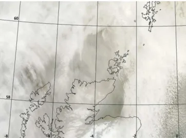
Figure 1.A high-resolution composite MODIS image of the semi-transparent cirrus case that occurred on 25 January 2010 located over north-east Scotland. The latitude and longitude grid is
super-imposed on the image showing latitude 58 to 60◦ (left side) and
longitude−8 to 0◦(bottom). The composite image was formed by
combining the MODIS red, green and blue channels to obtain the closest “true” colour image. The image is from the NERC Satel-lite Receiving Station, Dundee University, Scotland (http://www. sat.dundee.ac.uk/).
brief description of the radiative transfer model is also given. The retrieval methodology is described in Sect. 4 and results are discussed in Sect. 5. Section 6 presents the conclusions of this study.
2 The cirrus case, numerical weather prediction model and aircraft instrumentation
The conditions required for this paper are that the cirrus should be sufficiently optically thick to allow for discrimina-tion between various randomisadiscrimina-tions of the ensemble model using PARASOL retrievals, the aircraft and satellite should be coincident, and there should be no underlying cloud or broken cloud fields. It is practically very difficult to obtain all these necessary conditions at the same time. The cirrus case occurred on 25 January 2010 off the north-east coast of Scotland, which is shown in Fig. 1. The figure shows a high-resolution MODerate Imaging Spectroradiometer (MODIS) composite image (Platnick et al., 2003) of semi-transparent cirrus obtained at 13:30 UTC. The semi-transparent cirrus can be clearly seen around the north-east coast of Scotland, whilst further to the east, lower level water cloud underlying the cirrus can be seen. At about the same time as the image shown in Fig. 1 was taken, the FAAM (Facility for Airborne Atmospheric Measurements) BAe-146 aircraft was measur-ing the same high-cloud field.
shown in Fig. 1 was sampled by the aircraft as part of the “Constrain” field programme (Cotton et al., 2013). In this paper, one case from the Constrain field programme is pre-sented. There were several other Constrain cirrus cases, but these did not meet the conditions necessary for this paper. This is because the other cases were either optically too thick, there was no coincidence between PARASOL and the air-craft, or there was substantial underlying cloud.
For the case presented in this paper, the aircraft sampled the cirrus between the latitudes of about 58 and 59◦N, and between the longitudes of about 2.5 and 4.5◦W. The air-craft in situ instrumentation measured the temperatures of the cloud top and base to be about−55 and−30◦C, respectively. The aircraft began sampling the cloud at 11:55:06 UTC, and finished the sampling at 15:49:44 UTC. During this sam-pling time, the aircraft flew three straight and level runs above the cloud, each of about 10 min duration, commenc-ing at 13:19:00 UTC, 13:27:42 UTC and 15:21:42 UTC, re-spectively. From the aircraft, a dropsonde (measures vertical profiles of temperature, pressure and relative humidity with respect to water) was released at 13:30:00 UTC. In this study, use is made of the aircraft data from the earlier two runs as well as the dropsonde measurements which were most closely related to the PARASOL overpass. Note also that there was an 8 min interval between the two earlier straight and level runs, during which time the aircraft was manoeu-vring into position. In this paper, use is made of observa-tions from four instruments deployed on the aircraft. The first two instruments were the active Leosphere ALS450 elastic backscatter lidar and the passive Airborne Research Interfer-ometer Evaluation System (ARIES).
The nadir-pointing lidar operates at 0.355 µm with an integration time of 2 s and a vertical resolution of 1.5 m (Marenco et al., 2011). Further averaging of the signals has been done at post-processing, bringing the temporal resolu-tion to 10 s (equivalent at aircraft science speed to a 1.5–2 km footprint) and the vertical resolution to 45 m. The volume ex-tinction coefficient is computed from the lidar returns using the Fernald–Klett method described in Fernald (1984) and Klett (1985), assuming a lidar ratio of 20 sr.
The ARIES instrument is fully described in Wilson et al. (1999), but, briefly, it is a modified Bomem MR200 inter-ferometer that measures infrared radiances between the wave numbers of 3030.303 and 500 cm−1at a spectral resolution of 1 cm−1. The interferometer is capable of multiple viewing
geometries both up and down as well as across-track. The nadir-pointing ARIES and lidar data used here are from the straight and level runs above the cirrus. The other two in-struments deployed on the aircraft were used to measure the in situ vertical profile of RHi, these were the General East-ern GE 1011B Chilled Mirror Hygrometer (GE) and the Flu-orescence Water Vapour Sensor (FWVS) fast Lyman-alpha hygrometer (Keramitsoglou et al., 2002; Fahey et al., 2009). The RHi field of the cirrus case, shown in Fig. 1, has been simulated using the Met Office high-resolution NWP model.
The NWP simulation of the RHi field was obtained using a high-resolution limited-area model nested inside a suite of coarser resolution models. The high-resolution domain had a horizontal grid spacing of approximately 1 km and received hourly lateral boundary conditions from a 4 km model on a larger domain. The 4 km model was nested inside a 12 km domain, which was in turn driven by an N216 global model forecast. The 1 km grid was centred on (58.60◦N, 6.45◦W) with 1024 points east–west and 744 points north–south and a zonal and meridional grid spacing of 0.0135◦. The model time step was 50 s and the vertical level set comprised 70 levels, with a grid spacing of approximately 250 m at the al-titudes of interest for this study.
The model is non-hydrostatic and employs the semi-Lagrangian advection scheme.
In terms of model physics, the model is broadly compara-ble to the version of the Met Office operational UKV fore-casting system that was used operationally until the autumn of 2011 (Lean et al., 2008). However, in an attempt to rep-resent the simulated cloud system as well as possible, the following changes were made to the ice cloud microphysics. Firstly, the ice particle size distribution (PSD) parameteri-sation was changed so as to be consistent with the PARA-SOL radiative retrievals (see Sect. 3 for details). Secondly, the mass–diameter relation of the ice crystals was taken di-rectly from the Constrain in situ measurements (Cotton et al., 2013), and is therefore a “best estimate” of this property for the simulated cloud system. For this paper, the NWP model was initialised at midnight on 25 January 2010, and the RHi forecast field was extracted from the model on the same day but at the 13:00 UTC time step.
Figure 2.The ensemble model as a function of ice crystal maximum
dimension,Dmax. The first element of the model is the hexagonal
ice column of aspect ratio unity (first top left), followed by the 6-branched bullet rosette (top centre), the 3-monomer hexagonal ice aggregate (top right), 5-monomer ice aggregate (first bottom left), 8-monomer ice aggregate (bottom centre) and the 10-monomer ice aggregate (bottom right).
3 Ice crystal model and definitions of single-scattering properties
3.1 Ice crystal model and the particle size distribution function (PSD)
The model of ice crystals used in this study was developed by Baran and Labonnote (2007), and it is referred to as the ensemble model of cirrus ice crystals. The model has previ-ously been fully described by Baran and Labonnote (2007), but a brief description is given here, and the model is shown in Fig. 2. The model consists of six elements. The first ele-ment is the hexagonal ice column of aspect ratio unity, and the second element is the six-branched bullet rosette. There-after, hexagonal monomers are arbitrarily attached as a func-tion of ice crystal maximum dimension, forming 3-, 5-, 8-and 10-monomer polycrystals. The ensemble model has pre-viously been shown to predict the volume extinction coeffi-cient, ice water content (IWC), and column-integrated IWC, as well as the optical depth of mid-latitude and tropical cir-rus to within current experimental uncertainties (Baran et al., 2009, 2011a, 2013). Moreover, the model also replicated 1 day of PARASOL cirrus observations of total reflectance, be-tween the scattering angles of about 60 and 180◦(Baran and Labonnote, 2007). It was further shown by Baran and Labon-note (2007) that the second randomised member of the en-semble model, randomised in such a way as to produce fea-tureless scattering matrix elements, replicated 1 day of the global linear polarised reflectance measurements at close to cloud top.
0 0.2 0.4 0.6 0.8 1
10 100 1000 10000
Ar
Diameter um
Field (2008) lower & upper range McFarquhar (2013) Heymsfield (2003) Ensemble members
Figure 3.The ensemble model area ratio, Ar, as a function of ice
crystal diameter orDmax. The key is shown on the upper right-hand
side of the figure. The members of the ensemble model are repre-sented by the filled cyan circles. The in situ observations are from Field et al. (2008) (red lines), where the plus and cross signs rep-resent the lower and upper range of those observations and those
ranges have an uncertainty of±30 %. The blue error bar
repre-sents the mean and range of observations taken from McFarquhar et al. (2013) and the purple error bars represent the uncertainty in the observations taken from Heymsfield and Miloshevich (2003).
±25 % for sizes greater than 3000 µm. The data from Field et al. (2008) were obtained in the tropics at ice crystal max-imum dimensions between about 200 and 10 000 µm, and in Fig. 3, the upper and lower bounds on the data from Field et al. (2008) are shown, but on those bounds there is an un-certainty of±30 %. Estimates of Ar for ice crystals within 20 µm <Dmax< 100 µm were reported by Nousiainen et al.
(2011) to be between 0.84 and 0.70 using tropical data, and the Arratios in that paper were based on models of Gaussian random spheres (Muinonen 2000).
To compare members of the ensemble model against the in situ-derived estimates of Ar, the maximum dimension is defined as follows. The maximum dimension of the hexago-nal column is literally its maximum dimension (McFarquhar et al., 2013). The maximum dimension of the six-branched bullet rosette, and other members of the ensemble, is defined as the maximum distance across the particle when projected onto a two-dimensional plane (Heymsfield and Miloshevich 2003; Field et al., 2008). The area ratio (Ar)of the second member of the ensemble model shown in Fig. 2 assumes it to be in random orientation, which is a reasonable assump-tion since for the bullet rosette there is little difference be-tween the projected areas if the particle is in random or pre-ferred orientation due to its symmetry. All other members of the ensemble are assumed to be horizontally oriented along their maximum dimension with respect to the incident ra-diation. The oriented members are randomly oriented about their other two angles in three-dimensional space, with re-spect to the polar angle, to obtain an average of the projected areas, and it is these averages that are plotted in Fig. 3. In calculating the averaged Ar values, the effect of shadowing is taken into account for each of the aggregated ensemble members. Figure 3 shows that the Arratio calculated for each member of the ensemble model is within the current exper-imental range of possible Ar values reported in the litera-ture. The area ratio of the five-monomer aggregate at about 2500 µm is larger relative to the other ice aggregates. This is due to the other aggregate members of the ensemble model being more longitudinally elongated. Figure 3 shows why the model, as demonstrated by previous studies, can predict the volume extinction coefficient and the optical depth of natu-rally occurring cirrus to within current measurement uncer-tainties. In principle, given appropriate weights applied to the ensemble model, the volume extinction coefficient can be calculated for any type of cirrus (Baran et al., 2009, 2011a, 2013), assuming a representative PSD is applied. Currently, the members of the ensemble model are distributed into six equal intervals of the PSD. However, this distribution of the predicted area throughout the PSD can change, given fur-ther information on the most general weights to apply to the model.
In this study, the PSD assumed is the moment estimation parameterisation of the PSD developed by Field et al. (2007), hereinafter referred to as F07. The F07 parameterisation re-lates the second moment (i.e. IWC) to any other moment via
a polynomial fit to the in-cloud temperature. The parameter-isation is based on 10 000 in situ measurements of the PSD, and the measurements were filtered using the method of Field et al. (2006) to reduce artefacts of ice crystal shattering at the inlet of the microphysical probes (Korolev et al., 2011), and the PSD was truncated at an ice crystal maximum dimension of 100 µm. The in situ observations were obtained from the mid-latitudes and tropics, at in-cloud temperatures between about−60 and 0◦C. The parameterisation does not ignore ice crystals less than 100 µm, but assumes that these ice crys-tals follow an exponential PSD. For ice crystal sizes greater than 100 µm, the parameterisation uses a gamma function, which was found to best fit the in situ-measured PSDs. The parameterisation adds together the exponential and gamma function to reconstruct the full PSD, given the IWC and in-cloud temperature. It has been previously shown that the F07 parameterisation is a good fit to in situ measurements of trop-ical and mid-latitude PSDs (Baran et al., 2011a; Furtado et al., 2014). Since the parameterisation fundamentally relates the second moment of the PSD to any other moment via the in-cloud temperature, in order to estimate representative PSDs, a mass–diameter relationship is required. In this pa-per, the ensemble-model-predicted mass–diameter relation-ship is used to generate the F07 PSDs. The ensemble model mass–diameter relationship was previously derived by Baran et al. (2011b), and in that paper it was shown that the ensem-ble model predicts the ice crystal mass of each particle to be given by 0.04 D2, where D is the maximum dimension of each ice crystal and the mass and D are in units of kg and m, respectively.. The ensemble model mass–diameter relation-ship is within the upper uncertainty of the Constrain-derived mass–diameter relationship derived by Cotton et al. (2013), and it is therefore representative of naturally occurring ice crystal mass. Furthermore, use is made of the F07 parameter-isation, as we wish to be consistent with the PSDs assumed in the NWP model cloud scheme used later in the paper. 3.1.1 The single-scattering properties
changed with respect to their original direction, with the re-sult that featureless scattering matrix elements are predicted. The values of distortion can be between 0 and 1, where 0 represents unperturbed scattering matrix elements, and these retain scattering features such as halo and ice bows. As the distortion is increased to higher values, the optical features are removed in order to produce featureless scattering ma-trix elements. The distortion method attempts to replicate the complex processes that may occur on and within ice crystals, which could lead to featureless phase functions. Other au-thors refer to distortion as “microscale surface roughness”. However, this description of surface roughness may not be accurate, as surface roughness can take on different forms (Mason 1971; Pfalzgraff et al., 2010; Bacon et al., 2003; Malkin et al., 2012). For instance, a theoretical electromag-netic study by Liu et al. (2013) has shown that the method of distortion does not accurately reproduce the scattering phase function at high values of idealised surface roughness. In this study, the method of distortion is merely used to randomise the ice crystal so that featureless scattering phase functions are produced.
Here the distortion parameter is assumed to have the val-ues of 0, 0.15, 0.25 and 0.4. The distortion value of 0.4 is also combined with embedding the ice crystal with spheri-cal air bubbles in order to achieve the maximum randomi-sation of the ice crystals so as to produce featureless phase functions. The upper distortion value of 0.4 was chosen as this was found to best fit 1 day of global POLDER-2 re-trievals of directional spherical albedo and measurements of the linearly polarised reflectance (Baran and Labonnote, 2006). For the most randomised case of assuming a distortion value of 0.4 and embedding the ice crystal with spherical air bubbles, the phase functions are calculated using the mod-ifications by Shcherbakov et al. (2006) applied to the ray-tracing code of Macke et al. (1996a). The statistics describ-ing the tilt angles were shown by Shcherbakov et al. (2006) to be best represented by using Weibull statistics, where the Weibull distribution is defined by the scale (i.e. the distor-tion as described above) and shape parameters. This finding was based on cloud chamber measurements of the angular scattered intensity from a collection of ice crystals at a visi-ble wavelength, and comparisons between measurements and ray-tracing results showed that the Weibull statistics were the better match to the measurements. Moreover, the choice of Weibull statistics is consistent with independent cloud cham-ber results found by Neshyba et al. (2013). For the most ran-domised case considered in this paper, the Weibull statistics are assumed to have the following scale and shape parameter values of 0.4 and 0.85, respectively, and for the spherical air bubble inclusions, a mean free path of 200 µm is assumed (Baran and Labonnote, 2007). The chosen values describ-ing the Weibull statistics are also consistent with the values derived from independent cloud chamber measurements re-ported in Neshyba et al. (2013).
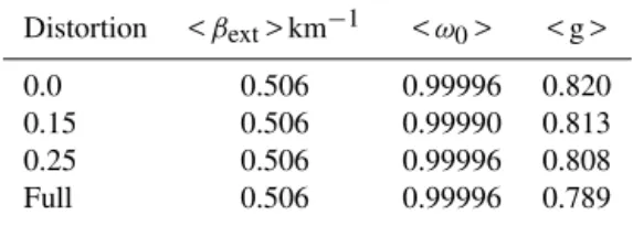
Table 1.The bulk values of <βext>, <ω0>andhgi, calculated at
the wavelength 0.865 µm, for each distortion, assumed to have val-ues of 0, 0.15, 0.25 and 0.4 plus spherical air bubble inclusions (Full).
Distortion <βext> km−1 <ω0> < g >
0.0 0.506 0.99996 0.820
0.15 0.506 0.99990 0.813
0.25 0.506 0.99996 0.808
Full 0.506 0.99996 0.789
To interpret the PARASOL measurements, the scatter-ing phase function is required. The bulk-averaged scatterscatter-ing phase function, < P11(θ )>, is given by the following
equa-tion:
hP11(θ )i =
R
Csca(q)P11(θ,q) n (q) dq
R
Csca(q) n (q) dq
, (1)
where the vector (q) represents the elements of the ensemble model as a function of maximum dimension,n(q) is the F07 parameterised PSD, and Csca(q) is the scattering cross
sec-tion of each of the ensemble model members. To generate the F07 PSDs, the IWC and in-cloud temperature are assumed to have the values of 0.01 gm−3and−50◦C, respectively.
The bulk-averaged asymmetry parameter,hgi, is calcu-lated using the following equation:
hgi =
R
g (q) Csca(q) n (q) dq
R
Csca(q) n (q) dq
. (2)
Another parameter of importance in calculating the total cloud reflectance is the single-scattering albedo,ω0, which
is the ratio of the scattered radiation to that completely at-tenuated in the hemisphere of all directions. Here, the wave-length of 0.865 µm is considered. At such a weakly absorbing wavelength the value ofω0will be close to unity.
The bulk-averaged volume extinction coefficient,hβexti,
is calculated from the following equation:
hβexti =
Z
Cext(q) n (q) dq, (3)
where Cext(q)is the extinction cross section of each member
of the ensemble model, calculated as a function of its maxi-mum dimension.
Figure 4. (a)The decadal logarithm of the ensemble model nor-malised scattering phase function as a function of scattering an-gle assuming a variety of distortions. The model cases shown are the pristine (black), slightly distorted (red), moderately distorted (dashed blue) and fully distorted with spherical air bubble inclu-sions (dotted purple).(b)The ratio between the distorted and pris-tine ensemble model phase functions as a function of scattering an-gle. Shown here are slight distortion (red), moderate distortion (dot-ted green) and full with spherical air bubble inclusions (dot(dot-ted blue). The key is shown in each of the figures.
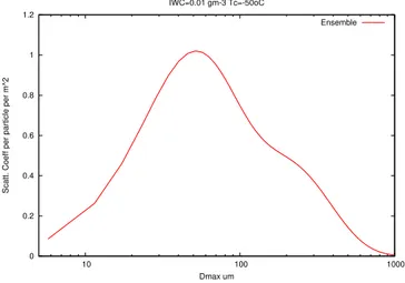
Figure 5 shows the maximum contribution to the ice crystal scattering cross section per particle, as a function of maxi-mum dimension, assuming the IWC and in-cloud tempera-ture values given above. The figure shows that the maximum contribution to the scattering cross section occurs at a max-imum dimension of about 50 µm. Defining the size param-eter,x, as πD/λ, whereλ is the incident wavelength, gives a value of x of about 182. This value of x means that the Monte Carlo ray-tracing method is within the range of x
where the method is applicable (Yang and Liou 1996). As stated previously, the methods adopted throughout this pa-per to represent ice crystal complexity have been applied to generate a range of phase functions that retain and re-move optical features that may be exhibited by naturally
0 0.2 0.4 0.6 0.8 1 1.2
10 100 1000
Scatt. Coeff per particle per m^2
Dmax um IWC=0.01 gm-3 Tc=-50oC
Ensemble
Figure 5.The scattering coefficient per particle (m−2)as a function
of ice crystal maximum dimension,Dmax. The PSD was generated
assuming IWC and in-cloud temperature values of 0.01 gm−3and
−50◦C, respectively.
due to the increasing values of the ratio at scattering angles between approximately 100 and 125◦, it might be possible to discriminate between models on a pixel-by-pixel basis at those particular scattering angles.
Of course, the phase functions derived from the ensemble model shown in Fig. 4 may not cover the entire range of pos-sible cirrus phase functions as there are many pospos-sible cirrus habits that might occur at particular environmental tempera-tures (see, for example, Baran, 2012, and references therein). However, in the case of aggregates of hexagonal plates or hexagonal columns, it was shown by Baran (2009), using the ice aggregation model of Westbrook et al. (2004), that after three monomers were attached to the ice aggregate, the asym-metry parameters and phase functions asymptote to their lim-iting values. This asymptote occurs because the ice aggrega-tion model predicts that the ice monomers making up the ice aggregate are well separated from each other. This separa-tion is sufficient to reduce the effects of multiple scattering on the phase function, resulting in only slight modifications to the scattering angle positions of optical features (see, for example, Fig. 5 and Fig. 6 of Baran, 2009). This aggrega-tion process is fundamental, and the same behaviour would be observed independent of the shape of the initial monomer (Westbrook et al., 2004). Therefore, in the case of pristine aggregates, the position of optical features on the phase func-tions would not be expected to be fundamentally different to those shown in Fig. 4a. If, on the other hand, the monomers that make up the ice crystal aggregate are sufficiently close to each other, then multiple scattering between monomers becomes important, as the scattered energy is increased and therefore also the phase function. However, the positions of the optical features exhibited by the ice aggregate phase func-tions do not significantly change position with respect to their scattering angles as these are principally determined by the
hexagonal geometry (Um and McFarquhar 2007, 2009). As discussed in the introduction to this paper, the observational evidence indicates that pristine ice crystals are a rarity in nature; therefore the phase functions of highly complex ice crystals exhibiting inclusions, cavities and surface roughness will produce featureless phase functions and the featureless nature of the phase function is invariant with respect to ice crystal habit.
To retrieve the spectral spherical albedo using PARASOL, a radiative transfer model is required; here the model de-veloped by de Haan et al. (1986) is used and its applica-tion to PARASOL has been fully described by Labonnote et al. (2001). The radiative transfer model assumes a plane-parallel cloud, but it is fully inclusive of multiple scatter-ing. Also taken into account are layers of aerosol below the cloud and Rayleigh scattering above and below the cloud is also taken into account. The aerosol model assumed in the PARASOL retrieval has been previously described by Buriez et al. (2005), and so a description will not be repeated here. However, the aerosol is principally maritime-based, and so its optical depth will be much smaller than the cirrus optical depth, and as such it will not be of any significance for the purposes of this paper. At the wavelength of 0.865 µm, the PARASOL retrieval algorithm assumes that the sea surface has a reflectance value of 0.000612 (the foam contribution outside of sun glint) and a wind speed of 7 ms−1. See Ap-pendix A in Buriez et al. (2005) for a detailed derivation of the assumed PARASOL sea surface reflectance value. The scattering by aerosol and ocean glint all contribute to the di-rectional variation of the retrieved cloud optical depth, and these effects are taken into account in the PARASOL re-trieval algorithm. In the next section, the rere-trieval method-ology is described.
4 Methodology
there is a one-to-one relationship between the cloud optical depth and the cloud spherical albedo (i.e. integral of the plane albedo over all incoming directions, where the plane albedo is a function of solar zenith angle alone) if the surface be-low the cloud is black. The cloud optical depth is retrieved by matching the simulated cloud reflectance to the measured cloud reflectance at each scattering angle. If the phase func-tion were a perfect representafunc-tion of the cloud, then the re-trieved cloud optical depth will be the same at each scattering angle. Therefore, the retrieved spherical albedo would also be the same at each scattering angle. If the assumed phase function were a poor representation of the cloud, then this would result in a directional dependence on the spherical albedo, which would be unphysical. This retrieval method-ology forms the basis of this paper, and it has been applied by other studies that have utilised PARASOL measurements to test ice cloud scattering phase functions (see, for exam-ple, Doutriaux-Boucher et al., 2000; Labonnote et al., 2001; Baran et al., 2001; Knapp et al., 2005; Baran and Labonnote, 2006).
As previously stated, the retrievals of spherical albedo are performed on a pixel-by-pixel basis, and the data products derived from the PARASOL observations are only used if the following four conditions are met: (i) for each 6 km×6 km pixel the cloud fraction is unity, (ii) the total number of view angles ≥7, (iii) the difference between the minimum and maximum sampled scattering angle is greater than 50◦, and (iv) only pixels over the sea are considered. The total num-ber of PARASOL pixels that are within the area of interest shown in Fig. 1 is 297. As previously stated, since the true cloud spherical albedo is, by definition, independent of di-rection, then for each pixel, the retrieved averaged directional spherical albedo,hSi, should be identical to the directional spherical albedo,S(θ), whereθis the scattering angle, if the model phase function were a perfect representation of the cloud. The retrievals ofS(θ) depend on the assumed scatter-ing phase function, the vertical volume extinction coefficient andω0.
The averaged spherical albedo,hSi, for each pixel is de-fined by
hSi = 1
N
j=N X
j=1
Sj(θ ) , (4)
whereN is the total number of viewing directions, which for the case considered in this paper is between 7 and 8. To find the phase function that best minimises the spherical albedo differences, the root-mean-square error (RMSE) is found for each pixel, which is given by
RMSE=
v u u u t
N P
j=1
1S2
N , (5)
where in Eq. (5),1S=hSi −S(θ). The RMSE is one gen-eral measure for choosing the best-fit model to the
observa-tions. However, once a set of RMSE minimisers has been identified, one should assess where the identification is sta-tistically significant. This is needed to rule out the possibil-ity that the differences in RMSE for the different distortions could have resulted from chance. To test this, we apply the Levene (1960) test statistic, as it is less sensitive to the condi-tion that the data must be normally distributed than the usual
F statistic, which is generally used to test whether the vari-ances between two samples are equal, provided the data fol-low a normal distribution. In the Levene test, the samples,k, are tested for homogeneity of variances between thek sam-ples. The total number of data points contained in all samples is given byN. The Levene null hypothesis is that variances betweenksamples are equal. The Levene null hypothesis is rejected, at some level of significance,α, if the Levene test statistic,W, is greater thanFα (k−1,N−k), which is the upper critical value of someF distribution withk−1 and
N−kdegrees of freedom. We consider pixels for which the derived RMSE values do not exceed 100 % to require test-ing for significance ustest-ing theW test. For these pixels, theW
test statistic is applied to test whether the model variances in1Sj are different at the 5 % significance level. If the null hypothesis is rejected, then that pixel is assigned a particu-lar model phase function. The 5 % orα=0.05 significance level is chosen, as this is simply betweenα=0.1 (10 %) and
α=0.01 (1 %) significance levels, so that the model test is neither too easy nor unrealistically hard, respectively.
In the sections that follow, the model phase functions shown in Fig. 4 and the total optical properties given in Ta-ble 1 are applied to the PARASOL measurements, on a pixel-by-pixel basis, to retrieve the phase function that best min-imises Eq. (5) and satisfies rejection of the Levene null hy-pothesis. Results of this analysis are then used to explore pos-sible relationships between the shape of the scattering phase function and RHi.
5 Results
5.1 Validating the NWP model field of RHi
Figure 6.The UKV-model-predicted field of the water vapour
mix-ing ratio (Qv)on 25 January 2010 at 13:00 UTC, between latitudes
57.8 and 59.7◦and longitudes−5.3 and−1.8◦. The units ofQvare
Kg Kg−1. The PARASOL pixels are represented by the open circles
and the aircraft track is represented by the solid line, and X marks the location where the aircraft was directly above the cloud at about 13:33:00 UTC.
field. From Fig. 6 we note that the NWP-model-predicted the cloud top to be in the vicinity of 10 km for the region of in-terest. Figure 7a shows the aircraft-mounted lidar estimate of the volume extinction coefficient as a function of altitude, and the bottom panel shows the derived lidar optical depth as a function of time. In Fig. 7a, note that only the lidar-derived profile of volume extinction coefficient greater than 6 km is shown. This is because, at altitudes less than this, the lidar equation becomes numerically unstable in clear air, and as such there were no meaningful retrievals of cirrus volume ex-tinction coefficient below this altitude. Figure 7a shows that the lidar-estimated cloud-top altitude was at about 10 km at approximately 13:33:00 UTC, which is in good agreement with the NWP model prediction, and the lidar position at that time is marked by the X symbol in Fig. 6.
To validate the NWP model prediction of the RHi field, use is now made of the aircraft-mounted ARIES measure-ments, which are applied to obtain retrievals of RHi. The re-trieval of RHi from the ARIES measurements is achieved using the Havemann–Taylor Fast Radiative Transfer Code (HTFRTC) (Havemann 2006; Havemann et al., 2009) and the retrieval method of Thelen et al. (2012). Moreover, the ARIES-based retrieval of RHi is validated against the drop-sonde measurements of RHi. The HTFRTC is a principal component based radiative transfer model and is fully
(a)
(b)
Figure 7. (a)The lidar-derived cloud volume extinction coefficient as a function of altitude (m) and time in units of hours after mid-night (UTC). The colour bar on the right-hand side of the figure indicates values of the cloud volume extinction coefficient in units of m−1, and the solid line represents the aircraft altitude.(b)The lidar-derived cloud optical depth from 300 m below the aircraft to the cloud base as a function of UTC time, and the horizontal solid line shown in the figure indicates an optical depth value of unity.
clusive of the atmosphere and exact multiple scattering. The ARIES spectrum was averaged over 10 spectra and was de-noised using principal components, which act as a low-pass filter. For this case, European Centre for Medium-Range Weather Forecasting (ECMWF) atmospheric profiles are ap-plied as the background state and the optimal estimation (OE) method of Rodgers (1976) is used, which is a Bayesian method. Here, OE is used to retrieve the most likely atmo-spheric state, and the method includes a rigorous treatment of error. The errors arise from the ARIES instrument itself and from the forward model, as well as from the ECMWF model background fields. The treatment of error by OE assumes that the errors are described by a Gaussian distribution. Here the background errors in the temperature, RH and IWC are as-sumed to be typically±0.4 K,±10 % and ±50 %, respec-tively. Given the errors, ARIES measurements and simulated measurements using HTFRTC, OE uses a minimisation pro-cedure to find the most likely atmospheric state that best de-scribes the measurement set, given the retrieved parameters or state vector. Currently, the state vector in the HTFRTC re-trieval method (Thelen et al., 2012) is composed of the tem-perature profile, the relative humidity profile, homogeneous cirrus IWC, surface temperature, and surface emissivity. The temperature and relative humidity profiles are retrieved at all 70 levels of the Met Office operational suite of models.
Figure 8.A comparison between the retrievals, dropsonde measurements, in situ measurements and NWP model predictions of RHi plotted
against the pressure (hPa) for two different locations.(a)The pixel located at longitude−3.84 and latitude 59.14◦and(b)the pixel located at longitude−3.20 and latitude 57.97◦. In(a)and(b), the retrievals are represented by the purple and green plus signs, dropsonde measurements are the solid grey line and filled grey circles, the General Eastern hygrometer is the solid green line, and the FWVS hygrometer is the solid red line.
in situ vertical profiles of RHi shown in the figures were obtained during an aircraft ascent from about 350 hPa to about 240 hPa, and the ascent started at 12:45:58 UTC and ended at 13:18:52 UTC. The dropsonde shown in the fig-ure was launched at 13:30:00 UTC. The ARIES retrievals of RHi took place whilst the aircraft was on a straight and level run above the cloud between the times of 13:19:00 and 13:32:13 UTC.
Figure 8a and b show that the two in situ RHi measure-ments are in good agreement with each other, whilst the dropsonde took some time to adjust to the prevailing atmo-spheric conditions. After this adjustment time, the infrared retrievals of RHi, in the presence of cirrus, are in good agree-ment with the dropsonde and are within the range of RHi measured by the two in situ instruments. The figure demon-strates that the retrieval of RHi using high-resolution pas-sive infrared measurements is sufficiently accurate and can be obtained, in the presence of cirrus, on a global scale using space-based high-resolution instruments such as the Infrared Atmospheric Sounding Interferometer (IASI). Furthermore, below the cloud, the dropsonde and retrievals are in very good agreement in the drier regions of the atmosphere, down to pressures of about 600 hPa. Moreover, the retrievals and dropsonde are in good agreement, down to pressures of about 1000 hPa. The two different retrieval colours represent the retrievals based on the two aircraft runs above the cirrus that were previously described. Each of the runs was 10 min in length. There were approximately eight ARIES retrievals per run. Figure 8 demonstrates that the retrievals, dropsonde
measurements and in situ measurements are sufficiently con-sistent to compare against the NWP model. Figure 8a shows the various comparisons at the latitude of 59.14◦N and lon-gitude 3.85◦W, which corresponds to the upper left of Fig. 6. The figure shows that the NWP model prediction of the ver-tical profile of RHi is consistent with the retrievals and mea-surements. Figure 8b is similar to Fig. 8a but for the location 57.97◦N and 3.20◦W, which corresponds to the lower left of Fig. 6. In this figure, the NWP model and retrievals can reach values of RHi of up to about 1.20. Figure 8a and b validate the NWP model prediction of RHi, and thus this model can be used to compare against the PARASOL estimates of ice crystal randomisation. Figure 8a and b show that the NWP-model-predicted cloud top is at about 200 hPa (∼10 km), and the cloud base is at about 400 hPa (∼7 km).
The NWP-model-predicted cloud depth is therefore about 3 km, which is also in good agreement with the lidar-derived maximum cloud depth shown in Fig. 7a at approximately 13:33:00 UTC, when the aircraft was above the cloud top. 5.1.1 Estimating the shape of the scattering phase
function and its relationship to RHi
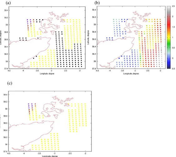
Figure 9.The PARASOL estimates of ensemble model randomisations (based on minimised RMSE) and retrievals of optical thickness as
a function of latitude and longitude.(a)The estimated ice crystal randomisation, where the indeterminate results are shown by the black
squares, the most randomised phase functions (distortion=0.4 with spherical air bubble inclusions) by the yellow squares, and the pristine phase functions (distortion=0) by the purple squares; dark- and light-brown squares represent the slightly distorted (distortion=0.15) and moderately distorted (distortion=0.25) phase functions, respectively.(b)The PARASOL-retrieved averaged optical thickness, averaged over all scattering angles, where the decadal logarithm of the retrieved optical thickness is shown by the colour bar on the right-hand side of the figure.(c)The same as(a)but with the indeterminate results removed.
estimates for each pixel, showing the phase function model that best minimised RMSE, are shown in Fig. 9a. The to-tal number of retrievals, showing only those retrievals over the sea, in Fig. 9a is 292. However, 130 of these retrievals correspond to indeterminate results. The reason for the in-determinate results at those pixels is because the retrieved spherical albedo at each of the scattering angles was the same for all ensemble models. The similarity of retrieved results in the indeterminate cases is because the retrieval conditions stated in Sect. 4 were not met. These indeterminate results are shown as black squares in the figure. A comparison be-tween Figs. 9a and 1 show that the indeterminate results gen-erally occurred in the presence of multi-layer cloud. Figure 9b shows the averaged retrieved PARASOL decadal optical thickness (averaged over all available scattering angles) at each of the pixels shown in Fig. 9a. The figure shows that the retrieved PARASOL optical thickness ranged between less than 1 and up to about 250. The largest optical
be-tween models will no longer be possible, and some of these largest optical thicknesses are associated with the indetermi-nate results. Figure 9c shows the estimated randomisations at each PARASOL pixel, but with the indeterminate results re-moved, again using only the minimised RMSE value to select the best model phase function. The yellow squares in Fig. 9c correspond to the most randomised phase function (i.e. dis-tortion=0.4 with spherical air bubble inclusions), and the number of pixels associated with this colour is 150, which, from the figure, is clearly the most common. However, 12 of the pixels shown in the top left of the figure are not associ-ated with the most randomised phase function. Rather, these pixels were found to be associated with the pristine phase function (distortion=0), the slightly distorted phase func-tion (distorfunc-tion=0.15), or the moderately distorted (distor-tion=0.25) phase function. The retrievals which best min-imised the RMSE assuming the pristine phase function are represented by the purple squares. The pixels represented by the dark- and light-brown squares were found to be associ-ated with the slightly (distortion=0.15) and moderately dis-torted (distortion=0.25) ensemble model phase functions, respectively. Therefore, the results shown in Fig. 9c indi-cate that, on a pixel-by-pixel basis, the most randomised ice crystal model phase functions may not always be the best fit to multi-angular spectral albedo measurements, at least if only the minimised RMSE value is used to select the best-fit phase function. Note, however, that we have so far disre-garded whether or not the discrimination of phase function, based on RMSE, is statistically significant. The reliability of the use of minimised RMSE values only to select the best model phase function is further examined in the paragraphs that follow.
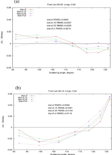
The estimated randomisations for two of the pixels shown at the top left of Fig. 9c are further examined in Fig. 10a and b. The figure shows the spherical albedo differences plotted as a function of scattering angle for each of the two pixels, and in each of the figures, the RMSE values are shown that were derived from the spherical albedo differences assuming the four models. The first pixel shown in Fig. 10a is located at latitude 59.03◦ and longitude−3.62◦, and this pixel has been assigned the fully randomised phase function. It can be seen from the figure that, in this case, the spherical albedo differences predicted by the fully randomised phase function are closer to the zero line than the other models for all scat-tering angles considered. In this case, the RMSE value found for the fully randomised model is a factor of 4.6 smaller than the value of the RMSE found for the pristine model. In con-trast to Fig. 10a, Fig. 10b shows the spherical albedo differ-ences for the pixel located at latitude 59.14◦ and longitude
−3.84◦, and this pixel has been assigned the pristine model phase function. In this case, the pristine model phase function is closest to the zero line at the scattering angles of about 92, 107 and 123◦. However, at the scattering angles of about 99 and 113◦, the pristine model phase function predicted spher-ical albedo differences are similar to the predictions obtained
Figure 10.Differences between the directionally averaged (<S>) and directional (S(θ )) spherical albedos as a function of scattering
angle at two pixel locations.(a)The spherical albedo differences
for the pixel located at 59.03◦and longitude−3.62◦, assuming the pristine ensemble model (dist=0) (open red circles), the slightly distorted model (dist=0.15) (open green triangles), the moderately
distorted model (dist=0.25) (open blue diamonds), and the fully
randomised model (dist=0.4 with spherical air bubble inclusions)
(open purple pentagons).(b)The same as(a)but for the pixel
lo-cated at latitude 59.14◦and longitude−3.84◦. The zero difference line is shown by the solid bold line, and the RMSE values calculated for each of the models are shown in each of the figures.
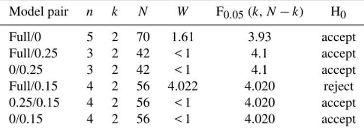
Table 2.The Levene test statistic,W, applied to test homogeneity of variances in spherical albedo differences between two groups of scattering phase function models for each set of pixels. In the table, the two phase function models are represented for each set of pixels by their assumed distortion values, referred to as Model pair; the total number of pixels used in each test isn. The null hypothesis is given by H0, which is either rejected or accepted;kis the number of
samples;Nis the total number of observations in the two samples;
and F0.05(k,N−k) is the value of the tabulated upper critical value
at the 5 % significance level composed ofkandN−kdegrees of
freedom.
Model pair n k N W F0.05(k,N−k) H0
Full/0 5 2 70 1.61 3.93 accept
Full/0.25 3 2 42 < 1 4.1 accept
0/0.25 3 2 42 < 1 4.1 accept
Full/0.15 4 2 56 4.022 4.020 reject
0.25/0.15 4 2 56 < 1 4.020 accept
0/0.15 4 2 56 < 1 4.020 accept
a non-featureless phase function was selected using the min-imised RMSE value test.
From Fig. 9c it can be seen that using minimised RMSE test, 5 of the 12 pixels are associated with pristine model phase functions (distortion=0), whilst 4 pixels are as-sociated with slightly distorted phase functions (distor-tion=0.15) and the other 3 pixels are associated with moder-ately distorted phase functions (distortion=0.25). All pixels associated with each of the above three distortion values were combined together. For each of the distortions, the W statistic was obtained in groups of two, so thatk=2. The variances in the spherical albedo differences obtained with the RMSE-determined best-fit phase function were compared against the variances obtained assuming all other model phase functions. For each group of two, the test W statistic was computed and then compared against the tabulated upper critical value of theFα (k−1,N−k) distribution in order to accept or reject the null hypothesis at the 5 % significance level. The results of this analysis are presented in Table 2.
In the case of the five pixels associated with pristine phase functions, it can be seen from Table 2 that the Levene null hypothesis must be accepted. Therefore, the variances in the spherical albedo differences determined using the RMSE best-fit model are not sufficiently different from the variances obtained using all other phase function models. A similar result to the above was found for the three pixels, which were associated with the moderately distorted phase function (distortion=0.25). For the four pixels associated with the slightly distorted model phase function (distortion=0.15), Table 2 shows that the null hypothesis can be rejected when its variances are compared against the variances obtained assuming the fully distorted model phase function (distor-tion=0.4 with spherical air bubble inclusions). However, for all other assumed models, for this group of four pixels, the
Table 3.Same definitions as Table 2 but with the Levene test statis-tic applied to a group of seven pixels, where the fully randomised model phase function was found to best fit spherical albedo dif-ferences using minimised RMSE values. The model pair tests are between all other scattering phase function models and the fully randomised scattering phase function model.
Model pair n k N W F0.05(k,N−k) H0
0/Full 7 2 98 18.289 3.93 reject
0.15/Full 7 2 98 19.436 4.1 reject
0.25/Full 7 2 98 12.918 4.1 reject
null hypothesis must be accepted. The results contained in Table 2 show that using minimised RMSE values alone may not be sufficient to select model phase functions on a pixel-by-pixel basis and that some other test statistic is required to compliment the RMSE method.
The Levene test statistic was also applied to some pixels associated with the most randomised phase function in order to test whetherW≫F for these pixels. The results of this test are presented in Table 3. In this case, seven pixels were se-lected between latitudes 57.92 and 58.92◦, and between lon-gitudes−3.42 and−3.71◦. As before, the seven pixels were combined, and the resulting variances in spherical albedo dif-ferences obtained assuming the most randomised phase func-tion were compared against the variances obtained assuming model distortion values of 0.15, 0.25 and 0. The results from Table 3 show that the null hypothesis can be very strongly rejected atα=0.05 (5 % significance level). The results of this analysis strongly suggest that the selection of the most randomised phase function using minimised RMSE values is acceptable, as illustrated by the example case in Fig. 10a.
the average of which is about 1.2. The lidar vertical profiles of optical depth were obtained when the aircraft was located above the cirrus, at an altitude of almost 11 km, which oc-curred during the times shown in the figure. There is a gap of about 3 min shown in Fig. 7b, which is the time required for the aircraft to turn and commence the second straight and level run. The PARASOL retrievals of cirrus optical thick-ness and the lidar retrievals are both consistent with one an-other. If there had been an underlying water cloud beneath the cirrus at the time of the PARASOL overpass, then the retrievals would not have been consistent. To examine the is-sue of underlying water cloud further, at a time nearer to the PARASOL overpass, generally available space-based cloud products were also examined.
The space-based remotely sensed cloud products are avail-able from http://www-pm.larc.nasa.gov/. The cloud prod-ucts that were examined were obtained at the time of 13:00:00 UTC, which is the time closest to the PARASOL overpass. The available remotely sensed cloud products from the site include detection of multiple cloud layers and cloud-top pressure. Analysis of these images indicated that the cloud overlying the 12 pixels was of a single layer, and the cloud-top pressure of this single-layer cloud was retrieved to be between 100 and 200 mbar (again not shown here for reasons of brevity). These independent space-based remote sensing results indicate that there was no underlying water cloud covering the 12 pixels, and this is consistent with the analysis of the high-resolution range-corrected lidar images as well as the PARASOL and lidar retrievals of cirrus optical depth.
Since it is unlikely that underlying water cloud affected the results discussed above indicates that there might have been backscattering structure present on the cirrus phase function which is not represented by any of the models. Or more sim-ply, there was insufficient scattering angle information avail-able to distinguish between models. Interestingly, Baran et al. (2012) also found that, for a case of mid-latitude, very high IWC anvil cirrus near to the cloud top, the PN-measured averaged scattering phase function also exhibited unusual backscattering features. Clearly, such findings of optical fea-tures on the scattering phase function of naturally occurring ice crystals indicate the need for radiometric or in situ ob-servations to sample the scattered angular intensities over a more complete range of scattering angle than is currently possible. Measuring the forward and backscattering inten-sities alone is not sufficiently general (Baran et al., 2012). However, the most common retrievals shown in Fig. 9a are representative of the most randomised ice crystals, and these have featureless phase functions. For the purposes of retriev-ing cirrus properties usretriev-ing global radiometric measurements, it is most likely that featureless phase functions are still gen-erally better at representing cirrus radiative properties than their purely pristine counterparts (Foot, 1988; Baran et al., 1999, 2001; Baran and Labonnote, 2006; Baum et al., 2011; Cole et al., 2013; Ulanowski et al., 2013; Cole et al., 2014).
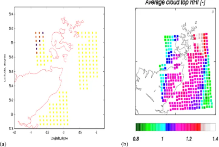
Figure 11.Associating the PARASOL estimations of shape of the scattering phase function at each pixel to the NWP-model-predicted field of RHi.(a)The estimated shape of the scattering phase
func-tion; the yellow squares are as previously defined in Fig. 9. The brown squares represent those PARASOL pixels where no phase function model could be assigned, and the blue squares represent those pixels where phase function models assuming distortion
val-ues of between 0 and 0.25 could be assigned.(b)The
NWP-model-predicted cloud-top RHi field, where the colour bar indicates the
range in predicted RHi.
Here, it is also of interest to note the change in the asym-metry parameter values shown in Table 1. From the pristine ensemble model phase function to the most randomised en-semble model phase function, the change in the asymme-try parameter is about 5 %. A change in the asymmeasymme-try pa-rameter of 5 % is radiatively important, as illustrated by the following example. Given that the instantaneous solar irra-diance arriving at the top of Earth’s atmosphere is about 1370 Wm−2. Under the assumptions of conservative scat-tering and a dark ocean below the cirrus, a change of 5 % in the asymmetry parameter results in a difference of about 43 W m−2 in the solar irradiance reflected back to space. However, the difference of 43 W m−2could be an underes-timate if actual values of the asymmetry parameter are lower than reported in Table 1 (Ulanowski et al., 2006). Even so, a difference of 43 W m−2 is very significant with regard to the energetics of the Earth’s atmosphere, and indicates why it is important to globally constrain values of the asymmetry parameter (Baran, 2012; Ulanowski et al., 2006, 2013; van Diedenhoven et al., 2014a).
Figure 12.The percent (%) probability of the penetration depth of solar radiation at 0.865 µm as a function of distance from the cloud top (km), and cloud optical depth for(a)forward-scattered and(b)
backward-scattered solar radiation in the principal plane, respec-tively. The percent probability of penetration is defined as the last position (distance from the cloud top) of the photon before leaving the cloud to reach the sensor. The cloud optical depth colour scale is defined by the key shown on the upper right-hand side of(a).
compared against the NWP-model-predicted RHifield at the cloud top, which is shown in Fig. 11b. The NWP model re-sults are shown at a cloud-top altitude of 10 km. On com-parison with Fig. 11a, it can be seen from Fig. 11b that the most randomised phase functions (i.e. yellow squares) generally correspond to model pixels with RHi> 1.0. Con-versely, the 12 pixels for which no one model phase function could be assigned generally correspond to NWP model pix-els with RHi< 1.0. The results for RHi> 1 are broadly con-sistent with the findings of Gayet et al. (2011) and Ulanowski et al. (2013). The results of the former paper suggested that featureless phase functions were generally associated with RHi> 1.0. Whilst the laboratory studies of Ulanowski et al. (2013), on ice crystal analogues, indicate that at higher levels of ice supersaturation, surface roughness on the ice crystal increased. This increase in surface roughness would naturally lead to featureless phase functions (Yang and Liou, 1998; Ulanowski et al., 2006; Baran, 2012; and references contained therein).
The NWP results shown in Fig. 11b are at the cloud top. However, the PARASOL retrievals might be based on re-flected solar radiation that comes from the extent of the cloud and not just from the cloud top. In reality, solar radiation at 0.865 µm will penetrate to some depth within the cloud layer, and this depth of penetration needs to be calculated to test whether the assumption of cloud-top penetration is correct.
To calculate the depth of penetrating radiation at 0.865 µm, a Monte Carlo radiative transfer model has been used to rep-resent the cirrus layer of relevance to this study. The Monte Carlo model used here is fully described by Cornet al. (2009). A description of the Monte Carlo model setup and
defini-tion of the probability of penetradefini-tion is given in Appendix A. The percent probability of penetration as a function of cloud depth and optical depth is shown in Fig. 12a and b. In the figures, the percent probability of penetration at 0.865 µm is defined as the last position (distance from the cloud top) of the photon before leaving the cloud to reach the sensor. Re-sults are shown in the figure for the forward- and backward-scattered radiation in the solar plane, respectively.
Figure 12a and b show that, by a depth of 1 km from the cloud top, the probability of penetration has been more than approximately halved for optical depths greater than 0.3. By 1.5 km from the cloud top, the probability of penetration is generally less than 5 %. The percent probability of penetra-tion shown in Fig. 12a and b is similar. This is because the scattering phase function used in the Monte Carlo calcula-tions, at backscattering angles, is largely invariant with re-spect to the scattering angle. This is simply because the scat-tering phase functions representing the most randomised ice crystals are flat and featureless at backscattering angles.
From Fig. 12a and b, it can be concluded that the PARA-SOL measurements of the total reflectance are biased to-wards the cloud top, and therefore comparison between the NWP model at the cloud top and PARASOL estimations of the shape of the scattering phase function is acceptable.
This paper has demonstrated the potential of using space-based remote sensing to investigate relationships between the scattering properties of ice crystals and atmospheric state parameters. However, one drawback of current space-based angle measurements is the limited range of multi-angle samplings: in this paper, only seven measurement an-gles were available. In regions where NWP model values of RHi were generally less than unity, it was impossible to as-sign a model phase function to the PARASOL observations. Clearly, if more multi-angle samplings were available, cou-pled together with a greater range of scattering angle, then discriminating between different phase function models may become more likely.
6 Conclusions
This paper has explored the relationship between RHi and the shape of the scattering phase function for one case of mid-latitude cirrus that occurred on 25 January 2010. This relationship has been explored by combining high-resolution NWP model RHi fields with satellite retrieval of the direc-tional spherical albedo at 0.865 µm. The satellite observa-tions were obtained from the PARASOL spherical albedo product at scattering angles between about 80 and 130◦. The satellite observations were analysed on a pixel-by-pixel ba-sis. It was found that featureless phase functions, represent-ing significant ice crystal randomisation, best minimised dif-ferences between the directionally averaged spherical albedo and the directional spherical albedo for about 90 % of the pixels for which discrimination was possible. However, for about 10 % of the pixels, it was found that discrimination be-tween model phase functions, based on spherical albedo dif-ferences, was not possible. In general, if multi-angular data are not available, given that over 90 % of the spherical albedo differences contained in this study were best described using featureless phase functions, then featureless phase functions are more likely to be a correct assumption for general appli-cation to the remote sensing of cirrus properties, rather than phase functions containing optical features.
It has also been demonstrated in this paper that the Met Office nested high-resolution NWP-model-predicted vertical profiles of RHi are sufficiently accurate to combine with remote sensing data to study relationships between atmo-spheric state variables and the fundamental scattering prop-erties of cirrus. Independent retrievals of the vertical profile of RHi, using aircraft-based high-resolution infrared data, dropsonde measurements and in situ measurements of RHi, showed excellent agreement with the NWP-model-predicted vertical profile of RHi for two very different locations within the cirrus field. Moreover, the NWP model prediction of cloud top, vertical depth and cloud base were shown to be consistent with lidar measurements of the same quantities. Assuming that the NWP RHi fields are representative of truth, the model fields were directly related to the remote sensing observations of the shape of the cirrus scattering phase function.
For this one cirrus case, it is found that featureless phase function models, representing highly randomised ice crys-tals, were shown to be generally associated with NWP model RHi values greater than unity. In the cases where the NWP model RHivalues were found to be generally less than unity, no one single-scattering phase function model could be as-signed to the PARASOL pixel using a quantitative statistical measure. The possibility of these pixels being affected by the issue of underlying water cloud below the cirrus was also investigated. Using high-resolution lidar images, retrievals of cirrus optical depth obtained from PARASOL and the aircraft-mounted lidar, and generally available space-based cloud products, it was found that it is unlikely that these pixels were affected by underlying water cloud. Given this finding, the model phase functions did not have the cor-rect structure in the backscattering part of the phase func-tion or, more simply, there was not enough scattering an-gle information to be able to discriminate more clearly be-tween the different phase function models. Given the latter reason, it would clearly be more desirable if future space-based instrumentation could more clearly resolve, and over a greater scattering angle range, the backscattering part of the cirrus phase function. This paper has also demonstrated that high-resolution interferometer data can be used, in the pres-ence of optically thin cirrus, to retrieve the vertical profile of RHi. This interferometric capability, which already exists in space through IASI, could be combined with improved res-olution of multiple viewing satellites to explore the relation-ship between atmospheric state parameters and shape of the scattering phase function on a global scale. This paper has demonstrated the potential for obtaining such global space-based measurements. There already exist aircraft-space-based in-struments that measure the in situ light-scattering proper-ties of atmospheric ice at particular locations, such as those used by Gayet et al. (2011), Ulanowski et al. (2013) and van Diedenhoven et al. (2014a). Preferably, new in situ instru-mentation should be developed that is capable of measuring the scattered intensities over a larger range of scattering an-gles than is currently possible (Baran et al., 2012).