www.nat-hazards-earth-syst-sci.net/12/927/2012/ doi:10.5194/nhess-12-927-2012
© Author(s) 2012. CC Attribution 3.0 License.
and Earth
System Sciences
A cautionary note regarding comparisons of fire danger indices
C. S. Eastaugh, A. Arpaci, and H. Vacik
Institute of Silviculture, Universit¨at f¨ur Bodenkultur (BOKU), Peter-Jordan Strasse 82, Vienna 1190, Austria Correspondence to:C. S. Eastaugh ([email protected])
Received: 10 August 2011 – Revised: 10 January 2012 – Accepted: 18 January 2012 – Published: 12 April 2012
Abstract. Over the past decade, several methods have been used to compare the performance of fire danger indices in an effort to find the most appropriate indices for particular re-gions or circumstances. Various authors have proposed com-parators and demonstrated different responses of indices to their tests, but rarely has much effort been put into demon-strating the validity of the comparators themselves. We present a demonstration that many of the published com-parators are sensitive to the different frequency distributions, that may be inherent in the performance of the different in-dices, and outline a non-parametric method that may be use-ful for future work. We compare four hypothetical fire dan-ger indices, three of which are simple mathematical trans-formations of each other. The hypothesis tested is that the comparators often used in such studies may indicate spuri-ous performance differences between these indices, which is found to be the case. Non-parametric methods are robust to differences in index value frequency distribution and may al-low more valid comparisons of fire danger indices. The new comparison method is shown to have advantages over other non-parametric comparators.
1 Introduction
Recently much effort has been put into finding the “best” fire danger indices for particular regions. Indices with greater skill may allow for more efficient allocation of firefighting re-sources, more appropriate public warning systems and more precise research studies. Regional differences in index per-formance may be apparent at relatively small geographical scales (e.g., Padilla and Vega-Garc´ıa, 2011), and it is un-likely that there will ever be a “one size fits all” approach. The United States Forest Service maintains the “FireFamily Plus” computer programme, one component of which can be used to analyse the performance of a range of fire danger in-dices (Andrews et al., 2003), and similar efforts to systemat-ically compare fire danger index performance are underway
in alpine Europe (e.g., Arpaci et al., 2010a, b). The compar-ison of fire danger indices is not trivial and the performance of indices must be tested according to high standards. Dif-ferent indices may be discrete or continuous and may pro-duce data across different ranges or follow different distribu-tions in their frequency of occurrence throughout a year, all of which serves to complicate direct comparisons.
1.1 Fire danger indices
The fire danger indices we are concerned with here are those formed so as to assign some particular value to any day, with (usually) higher values indicating a greater chance of a fire occurring. These indices form the basis of public warning systems and are of increasing interest for fire planning and resource allocation.
A wide variety of indices have been developed, with differ-ent mathematical formulations and differdiffer-ent input variables. Some of these use only the weather conditions on the days in question, such as the Angstr¨om index (IA), which is
depen-dent only on the relative humidity (R, %) and the temperature (T,◦C):
IA=
R 20+
29−T
10 (1)
(note that in this case, lower values indicate higher fire dan-ger).
Other indices also include information from previous days. The Nesterov index (IN) is constructed using temperature
and the dew point (D,◦C), summed over the number of days since a rainfall of 3 mm was recorded (W):
IN=
W
X
i=1
Ti(Ti−Di) (2)
1.2 Parametric and non-parametric tests
Parametric statistical tests assume by definition that data fol-lows some particular statistical distribution and are often in-valid if those assumptions are not met. Although for some tests these conditions are well known (such as the assump-tion of a normal distribuassump-tion in the calculaassump-tion of t-tests), in complex procedures or statistical software packages the need for the data to meet certain conditions may not be imme-diately apparent. Consequently, the ensuing results are at best meaningless, or at worst dangerously misleading. Ex-ploratory data analyses should always be performed before applying complex statistical procedures.
Using a simple set of hypothetical indices, we show here that these differences in frequency distributions can intro-duce spurious results into common index comparison meth-ods. A non-parametric test (not affected by differences in frequency distribution) is introduced which can support com-parative studies in future research. Although this paper serves to introduce the new method to the scientific commu-nity for further study, our main purpose is to elucidate the shortcomings of methods currently in use and, thus, demon-strate the necessity for the development of more descriptive non-parametric index comparison methods.
1.3 Previous approaches
Over the past decade or so several methods have been pro-posed to compare fire danger indices. For reasons of space these methods are only briefly described here; readers are asked to refer to the cited papers.
1.3.1 Mahalanobis distance
The Mahalanobis distance is a measure of the distance be-tween two datasets. Viegas et al. (1999) applied this method in southern Europe, beginning by normalising their indices so that all will range from zero to 100. This is done linearly, with the normalised index
Ix′ =100(Ix−Imin)/(Imax−Imin) (3)
whereIx′ is each individual normalised index value, Ixis the individual index value at its original scale Iminis the minimum value ofIxin the full dataset, and Imaxis the maximum value ofIxin the full dataset. The normalised indices are then grouped into ten cate-gories (Ix′ =0:10, 10:20 etc.). Viegas et al. (1999, p. 240) recognised the possibility of error being introduced due to using equally spaced class limits, but proceeded due to the simplicity of this approach. After plotting the percentage of days in each class and the percentage of fire-days in each class, they calculated the Mahalanobis Distance (Md)as a
measure of the discrimination of days with higher or lower fire danger. The Mahalanobis Distance is calculated as:
Md= [(X1−X2)/σ]2 (4)
whereX1 is the mean index value on fire-days, X2 is the
mean index value on non-fire days andσ is the standard de-viation of the index value on all days. A larger Mahalanobis Distance is presumed to represent greater differentiation of fire/nonfire-days. Note also that Md gives the same result
whether raw or normalised index values are used. 1.3.2 Percentile analysis
Andrews et al. (2003) described a “percentile analysis”, where, for a particular index, the index values at the 90th, 50th and 25th percentile are calculated for all days and com-pared with the corresponding percentile of that index value on fire-days. For example, the 90th percentile of some index across all days may have a value of 80, but when consider-ing only fire-days a value in that index of 80 represents the 75th percentile, a difference of 15. The differences for each of the three given percentiles are summed and represent the shift in the distribution of index values between all days and fire-days. A greater distribution shift is taken to signal a bet-ter index. Using the 90th, 50th and 25th percentiles appears to be subjective; selecting a different set of percentiles would give different results.
1.3.3 Logistic regression
As the occurrence or non-occurrence of a fire is a binary event, it may be modelled with a logistic regression. An-drews et al. (2003) also used a logistic regression technique to model the probability of a day at a particular index value being a fire-day or a nonfire-day with the index values as independent variables. The indices are ranked according to the range of the fitted values (with wider ranges, beginning closer to zero being indicative of more sensitive models) and to the fit of the models to the observations using a pseudoR2 value that they denoteRL2. A higherRL2indicates a closer fit of the logistic regression to the observed data.
1.3.4 c-index
Verbesselt et al. (2006) also used a logistic regression model, but judged their models’ performances using an adjusted chi-square form of Akaike’s Information Criteria (AIC), where AICχ2is the model likelihood ratio chi-squared statistic
●
●
●
0
20
40
60
80
100
Fire rank
P
er
centile on fire da
y
0 1 2 3
94.24 90 Y
31.64 50 n
34.08 60 Y
30.21 30 n
72.05 70 n
21.54 20 n
4.53 0 n
31.5 40 n
80.18 80 Y
13.75 10 n
Index.value Percentile Fire.Day
Fig. 1. Example figure for the proposed ranked percentile method of index comparison. Fire danger index values for every day are expressed as percentiles and those percentiles on days when fire occurs are plotted according to rank. The slope and intercept of a robust regression line through these points characterises the index.
at or above that value) and its “specificity” or “false posi-tives” (the index’s propensity for false alarms at or below that value). Fawcett (2006) provides an excellent overview of the concept and notes that the area under the curve is equiva-lent to a non-parametric Wilcoxon test of ranks (Hanley and McNeil, 1982). A c-index of less than 0.5 indicates random predictions, whereas a “perfect” model would have a c-index of 1.0.
The c-index gives useful non-parametric information, but is not adequate to fully describe differences in the perfor-mance of competing indices. Two ROC curves may not be identical, yet have the same area beneath them.
2 Methods
2.1 Proposed new comparator
We present here an outline of a two-part descriptor of fire in-dices that may help to differentiate performance, based on the slope of the ranked fire-day percentiles and the “y” intercept of that slope. The daily values for each index are converted to individual percentiles across the full range of days in the dataset. Those index percentiles for fire-days are ranked from lowest to highest and plotted on the “y”-axis, with the “x”-axis indicating the rank. Figure 1 provides a small example, with three fires occurring within a timespan of ten days.
Considering that on this plot an index composed of ran-dom numbers would have an expected slope of 1.0 and an intercept of zero while a “perfect” index would have a slope
approaching zero and an intercept approaching 100, these two parameters together may usefully describe the perfor-mance of fire indices. To reduce the influence of outliers in the data, the slope is calculated with the Theil-Sen tech-nique (Theil, 1950; Sen, 1968), which gives the median of all slopes from all points plotted to all other points. The inter-cept is the median of all of the possible individual interinter-cepts of that slope, passing through each single point. Although the Theil-Sen method is well established in the hydrological sciences as a means of producing a robust regression (e.g., Granato, 2006), to the best of our knowledge we are the first to suggest that it may be applied in order to characterise a curve of ranked percentiles, and that such a curve can use-fully describe the performance of a fire danger index. 2.2 Test and application example
To assess the robustness and usefulness of these index com-parison methods, we firstly constructed a set of four hypo-thetical indices and applied them to a arbitrary year con-taining 10 fire days. The four hypothetical indices were as-sessed with the four previously published comparison meth-ods and with our proposed new comparator. This is intended to demonstrate the need for non-parametric techniques.
The greater utility of our ranked-percentile method is shown through a brief application example. Meteorological data was obtained from the weather station in Graz (south-ern Austria) and used to derive values for the Angstr¨om and Nesterov indices for the surrounding region over the period 1978–2008. Twenty-one fires occurred in this time period. This data is a subset of an Austria-wide project examining the performance of 19 different indices including, for exam-ple, the Canadian FWI (Van Wagner, 1987), the M68 index (K¨ase, 1969) and the FMI of Sharples (2009).
Calculations of the hypothetical index values, the Maha-lanobis Distance and the percentile scores for the theoretical examples in this paper were made in Excel 2003, and both these and the remaining tests were performed with the R sta-tistical software v.13.1 (R Development Core Team, 2008), using the “glm” model (“binomial” family) to develop the lo-gistic regressions, the “anova” function to derive the model likelihood ratio chi-squared statistic to calculate AIC and functions in the “pROC” package (Robin et al., 2011) to cal-culate the c-index and the “mblm” package for the Theil-Sen statistics. The use of both Excel and R is intended to explore what differences may potentially result from applying the tests under different software frameworks. R and all pack-ages used are available via http://cran.r-project.org/. Calcu-lations for the Graz application case are made solely in R. 2.3 Index value generation
0 100 200 300 400
0
20
40
60
80
Day
Inde
x A
0 100 200 300 400
−4
−2
0
2
4
Day
Inde
x B
0 100 200 300 400
0
5000
15000
Day
Inde
x C
0 100 200 300 400
0
20
40
60
80
Day
Inde
x D
Fire
Fig. 2.Hypothetical fire danger index values over the course of one year. Index A is sinusoidal, as defined in Eq. (5) (in text). Indices B and C are respectively logarithmic and exponential transformations of index A, and index D is a discontinuous function described in Equation set 6 (in text). Triangles indicate fire occurrence days.
A=sin
3π 2 +
2dπ 365
×50+50 (5)
with d being the day of year and the sin calculated with radians. The index is thus sinusoidal with a period of one year and a range of zero to 100. Two further indices are constructed as transformations of the first, with index “B”=ln(A)and index “C”=eA/10. Finally, index “D” is independent and discontinuous, with:
D[d=1:d=57] =0,
D[d=58:d=168] =(d−58)/1.1, D[d=169:d=247] =(294−d)×0.8,
D[d=248:d=365] =(365−d)/(365/116). (6) Ten days are arbitrarily selected as “fire occurrence” days, 9 loosely centred around the middle of the year and one out-lier. For this example, these are days 4, 143, 156, 170, 189, 201, 208, 222, 247 and 262.
2.4 Index characteristics
Figure 2 displays the daily values of the four indices and the fire occurrence days, while Fig. 3 shows the frequency dis-tributions over all days. Index A values occur mostly at each extreme, while the mathematical transformations applied to create indices B and C causes the distributions to cluster to-wards one extreme.
Index A
0
20
60
100
0
15
Index B
−10
−5
0
5
0
40
Index C
0
10000
20000
0
100
Index D
0
20
60
100
0
30
Fig. 3.Frequency distributions of the four hypothetical indices.
As the first three indices are simply mathematical trans-formations of each other (i.e., ranks are not changed through the transformation), it is reasonable to suppose that any valid method of comparing them should rank each index as equally useful, otherwise the comparison method may be ranking in-dices differently simply because the index values have dif-ferent occurrence frequency distributions. This proposition will be tested for a number of different comparators that have been proposed in the literature, following procedures described by Viegas et al. (1999), Andrews et al. (2003) and Verbesselt et al. (2006).
3 Results
3.1 Hypothetical indices
0 20 40 60 80 100
0
20
60
P
er
centa
g
e of all da
ys
Index A Index B Index C Index D
0 20 40 60 80 100
0
5
10
20
Normalised index class
P
er
centa
g
e of fire da
ys
Fig. 4. Characteristics of normalised indices. Top figure shows the percentage of days falling in each index class, while the bottom figure is the percentage of the days in each class that recorded a fire occurrence.
shows little consistency between indices with regard to which “normalised” index class contains the highest proportion of fires.
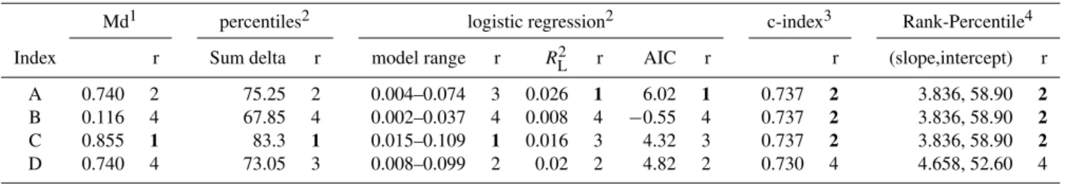
Results for the Mahalanobis Distance, the percentile anal-ysis, logistic regression statistics and the c-index are given in Table 1, along with the ranks of each index for each compara-tor. The only comparator that detects that indices A, B and C are effectively identical is the c-index. Also, c-index re-sults are identical whether calculated using raw index values, “normalised” values or fitted values from the logistic regres-sion, because the indicator uses ranks rather than values.
Ranking the fire-day percentiles of each index gives iden-tical results for indices A, B and C, but some differences are apparent to index D (Fig. 5). Index D performs better at the fifth and tenth ranks, but poorer at all others. The Theil-Sen robust regression line summarises the performance dif-ference, with indices A, B and C having a slope of 3.836 and an intercept of 58.90, and index D having a slope of 4.658 and an intercept of 52.60. Index D is, thus, concluded to have less skill than the others, which are of equal worth. 3.2 Application example
The results for the Graz application example are shown in Table 2. The c-index suggests that the indices are identi-cal, while other methods may recommend either. The ranked percentile curves are shown in Fig. 6, demonstrating that the performances of the two indices are in fact different.
0 2 4 6 8 10
0
20
40
60
80
100
Rank
Inde
x per
centile score on fire−da
y
* *
* *
* * * *
* *
Indices A, B and C
* Index D
Fig. 5.Robust regression of ranked percentiles.
0 5 10 15 20
0
20
40
60
80
100
Rank
Inde
x per
centile score on fire−da
y
* * *
* * * * * * * *
* *
* * * * * * * *
Angström
* Nesterov
Fig. 6. Ranked percentile curve for the Angstr¨om and Nesterov indices, applied to the 21 fires that occurred in the Graz region, 1978–2008.
4 Discussion and conclusions
Table 1. Comparator values and ranks for each index applied to the 4 hypothetical indices. Md=Mahalanobis distance;RL2=PseudoR2, as per Andrews et al. (2003); AIC=Akaike’s Information Criteria, r=rank. Bold numbers in the rank column indicate the “best” index according to each method
Md1 percentiles2 logistic regression2 c-index3 Rank-Percentile4
Index r Sum delta r model range r RL2 r AIC r r (slope,intercept) r
A 0.740 2 75.25 2 0.004–0.074 3 0.026 1 6.02 1 0.737 2 3.836, 58.90 2
B 0.116 4 67.85 4 0.002–0.037 4 0.008 4 −0.55 4 0.737 2 3.836, 58.90 2
C 0.855 1 83.3 1 0.015–0.109 1 0.016 3 4.32 3 0.737 2 3.836, 58.90 2
D 0.740 4 73.05 3 0.008–0.099 2 0.02 2 4.82 2 0.730 4 4.658, 52.60 4
1Viegas et al. (1999);2Andrews et al. (2003);3Verbesselt et al. (2006);4this study.
Table 2.Comparator values and ranks for each index applied to Angstr¨om and Nesterov indices in the Graz area. Bold numbers in the rank column indicate the “best” index according to each method.
Md percentiles logistic regression c-index Rank-Percentile
Index r Sum delta r model range r R2L r AIC r r (slope,intercept) r
Angstr¨om 1.053 2 119.92 1 0.000–0.029 2 0.011 1 26.79 1 0.816 1.5 2.350, 57.79 2 Nesterov 1.598 1 95.69 2 0.001–0.090 1 0.005 2 15.94 2 0.816 1.5 1.981, 63.28 1
0 200 400
0
20
40
60
80
100
Day
Normalised inde
x v
alue
a
0 200 400
Day
90
98
99
100
Index A B Fire
b
Fig. 7.Hypothetical fire danger index values over the course of one year, on linear(a)and exponential(b)“y”-axes.
days. Consider though, if the y-axes on the plots were dis-played on a different scale. Figure 7b shows the identical in-dices on an exponential scale. The data and the relationship between each index and the day of year is identical to that in Fig. 7a, only the scale of the “y”-axis is changed. Yet now, it “appears” that index B has greater discriminatory power than index A, because index A is commonly low on fire days.
The parametric methods examined in this paper are essen-tially Euclidean distance-based, in linear space. As pointed out by Wu (2005), there is no a priori reason to suppose that linear scaling is necessarily superior. The differences that some comparators find between the transformed indices are a result of the distribution, just as the appearance in Fig. 7 is the result of the axis scale.
Apart from the c-index, all of the established fire index comparators that we examined here indicate different predic-tive power between the effecpredic-tively identical indices A, B and C, suggesting that in many cases the differences they detect are spurious, resulting from the frequency distributions of the index values rather than from any real difference in predictive power.
methods involve some degree of interpolation between data points. In practical applications (with large numbers of fire-days) this particular shortcoming of the method is unlikely to cause problems if R is used rather than Excel, but may be im-portant where smaller numbers of events (such as “multiple fire-days” or “large fire days”) are of interest. The choice of which quantiles to be compared is somewhat subjective and will sometimes influence the results of the comparisons. In our Graz application example, the percentile analysis method suggests that the Angstr¨om index is substantially better than the Nesterov (Table 2). The reason for this is apparent in Fig. 6. The 90th, 50th and 25th percentiles are used for com-parison. While at the 50th and 25th percentile the curves for the two indices are at similar points, at the 90th percentile the Angstr¨om curve is higher. If the 75th percentile had been used instead of the 90th, the percentile analysis method would have determined the Nesterov to be the better index.
The non-parametric method that we outline appears to avoid some of the shortcomings of parametric methods, cor-rectly determining that the hypothetical indices A, B and C have equal predictive power. The method is in agreement with the c-index, that index D is inferior to the other indices. The proposed method also offers an improvement over the c-index, in that it is able to distinguish differences between fire indices that have identical c-index scores, where such dif-ference is real rather than an artefact of frequency distribu-tion. Our Graz application case was selected to demonstrate this. The c-index for both the Angstr¨om and Nesterov in-dices is 0.816, yet the ranked percentile curves for each index have different characteristics. The higher intercept and flatter slope would lead us to accept the Nesterov as the better in-dex in this application. Although from Fig. 6, we can see that the Angstr¨om works well at the very high values (above the 90th percentile), its performance below this level is compar-atively poor, with several fires occurring when the index was between its 66th and 76th percentile levels. The Nesterov index for fires at the same ranks was between its 72nd and 79th percentiles. This is immediately clear from the figure, but this pattern is also inferable from the fact the Angstr¨om index has a lower intercept and a higher slope than the Nes-terov.
Although substantial work remains to be done on deter-mining acceptable methods for comparing fire indices, we have established that commonly used parametric methods may produce potentially spurious results. Our proposed two-part non-parametric comparator is robust to index dis-tribution differences and can provide more useful informa-tion than current alternatives. Future investigainforma-tions will be needed to determine its full worth, including indepth mathe-matical analyses and application studies over a range of real-world datasets.
Acknowledgements. This research has been conducted partly within the frame of the Austrian Forest Research Initiative (AF-FRI), which is funded by the Austrian Science Fonds (FWF) with the reference number L539-N14 and the European Project ALP FFIRS (Alpine Forest Fire Warning System), which is funded by the European Regional Development fund of the Alpine Space Program with the reference number 15-2-3-IT. We also acknowledge the helpful comments provided by participants at the 2011 European Geosciences Union general assembly, where a pr´ecis of this work was presented (Eastaugh et al., 2011). Insightful comments from three anonymous reviewers served to substantially improve the paper.
Edited by: R. Lasaponara
Reviewed by: three anonymous referees
References
Andrews, P. L., Loftsgaarden, D. O., and Bradshaw, L. S.: Evalu-ation of fire danger rating indexes using logistic regression and percentile analysis, Int. J. Wildland Fire, 12, 213–226, 2003. Arpaci, A., Beck, A., Formayer, H., and Vacik, H.: Interpretation
of fire weather indices as means for the definition of fire dan-ger levels for different eco-regions in Austria, 6th international conference on Forest Fire Research, Coimbra, Portugal, 15–18 November, 2010, BP12, 2010a.
Arpaci, A., Vacik, H., Formayer, H., and Beck, A.: A collection of possible Fire Weather Indices (FWI) for alpine landscapes, avail-able at: http://www.alpffirs.eu/index.php?option=com docman\
&task=doc download\&gid=240\&Itemid=21\&lang=en (last access: 6 March 2012), 2010b.
Eastaugh, C. S., Arpaci, A., and Vacik, H.: Methods of comparing fire danger indices. European Geosciences Union general assem-bly, Vienna, Austria, 3–8 April 2011, EGU2011-9470, 2011. Fawcett, T.: An introduction to ROC analysis, Pattern Recogn.
Lett., 27, 861–874, 2006.
Granato, G. E.: Kendall-Theil Robust Line (KTRLine – version 1.0) – A visual basic program for calculating and graphing ro-bust nonparametric estimates of linear-regression coefficients be-tween two continuous variables: Techniques and Methods of the US Geological Survey, book 4, chap. A7, 31 pp., 2006. Hanley, J. A. and McNeil, B. J.: The meaning and use of the area
under a Receiver Operating Characteristic (ROC) curve, Radiol-ogy, 143, 29–36, 1982.
Hyndman, R. J., and Fan, Y.: Sample quantiles in statistical pack-ages, Am. Stat., 50, 361–365, 1996.
K¨ase, H.: Ein Vorschlag f¨ur eine Methode zur Bestimmung und Vorhersage der Waldbrandgef¨ahrdung mit Hilfe komplexer Kennziffern, Akademie Verlag, Berlin, 68 pp., 1969.
Padilla, M. and Vega-Garc´ıa, C.: On the comparative importance of fire danger rating indices and their integration with spatial and temporal variables for predicting daily human-caused fire occur-rences in Spain, Int. J. Wildland Fire, 20, 46–58, 2011.
R Development Core Team: R: A language and environment for statistical computing, R Foundation for Statistical Computing, Vienna, Austria, 2008.
S+ to analyze and compare ROC curves, BMC Bioinformatics, 12, p. 77, 2011.
Sen, P. K.: Estimates of Regression Coefficient Based on Kendall’s tau, J. Am. Stat. Assoc., 63, 1379–1389, 1968.
Sharples, J. J., McRae, R. H. D., Weber, R. O., and Gill, A. M.: A simple index for assessing fire danger rating, Environ. Model. Softw., 24, 764–774, 2009.
Theil, H.: A rank invariant method for linear and polynomial re-gression analysis, Nederlandse Akademie van Wetenschappen Proceedings Series A, 53, 386–392 (Part I), 521–525 (Part II), 1397–1412 (Part III), 1950.
Van Wagner, C. E.: Development and structure of the Canadian for-est fire weather index system, Canadian Forfor-est Service, Ottowa, 48 pp., 1987.
Verbesselt, J., J¨onsson, P., Lhermitte, S., van Aardt, J., and Coppin, P.: Evaluating satellite and climate data-driven indices as fire risk indicators in savanna ecosystems, IEEE T. Geosci. Remote, 44, 1622–1632, 2006.
Viegas, D. X., Bovio, G., Ferreira, A., Nosenzo, A., and Sol, B.: Comparative study of various methods of fire danger evaluation in southern Europe, Int. J. Wildland Fire, 9, 235–246, 1999. Wu, L.: Automated modeling and nonlinear axis scaling, Ph.D.