Population Genetic Analysis of Colombian Trypanosoma cruzi Isolates Revealed by Enzyme Electrophoretic Profiles

(1)

31 31 31 31 31 Mem Inst Oswaldo Cruz, Rio de Janeiro, Vol. 96(1): 31-51, January, 2001

Population Genetic Analysis of Colombian

Trypanosoma

cruzi

Isolates Revealed by Enzyme Electrophoretic Profiles

Manuel Ruiz-Garcia/

+

, Marleny Montilla, Sebastian Nicholls, Diana Alvarez

Unidad de Genética (Genética de Poblaciones-Biología Evolutiva), Departamento de Biologia, Facultad de Ciencias, Pontifica Universidad Javerina, Cra 7A No. 43-82, Bogotá DC, Colombia *Instituto Nacional de Salud,

Laboratorio de Parasitología, Bogotá DC, Colombia

Although Colombia presents an enormous biological diversity, few studies have been conducted on the population genetics of Trypanosoma cruzi. This study was carried out with 23 Colombian stocks of this protozoa analyzed for 13 isoenzymatic loci. The Hardy-Weinberg equilibrium, the genetic diversity and heterogeneity, the genetic relationships and the possible spatial structure of these 23 Colombian stocks of T. cruzi were estimated. The majority of results obtained are in agreement with a clonal population structure. Nevertheless, two aspects expected in a clonal structure were not discovered in the Colombian T. cruzi stocks. There was an absence of given zymodemes over-represented from a geographical point of view and the presumed temporal stabilizing selective phenomena was not observed either in the Colombian stocks sampled several times through the years of the study. Some hypotheses are discussed in order to explain the results found.

Key words: Trypanosoma cruzi - population genetics - spatial autocorrelation - Colombia

In the present study, we show an extensive population genetics analysis, where the genetic

heterogeneity and the spatial structure of

Trypa-nosoma (Schizotrypanum) cruzi is analyzed throughout Colombia. This kind of study is of clini-cal importance since the extensive genetic poly-morphism and heterogeneity of isolates may be re-lated to the diverse pathology of the disease and its immunity, throughout the geographical distri-bution of the clonets (Dvorak 1984, Cosenza & Kroeger 1991). Although well kown in other Latin American countries (Brazil, Bolivia, Chile, for ex-ample), some population and spatial patterns of the

T. cruzi clonets in Colombia are not very well known. The only previous studies reported for this coun-try were those from Saravia et al. (1987), where 47 stocks were analyzed coming from the Piedmont region (Meta and Casanare departments); the in-clusion of five Colombian stocks (MC50, MC52, MC53, MC60 and MC61) belonging exclusively to one zymodeme (19) in the study of Tibayrenc and Ayala (1988) and, more recently, the work of Márquez et al. (1998), where 28 new stocks coming

from the Sucre, Antioquia and Tolima departments were analyzed. In the first work, 12 different zymodemes were detected (12/47 = 25.5%). In the second, the genetic variability shown in Colombia was lower, because only one zymodeme was de-tected from the five stocks analyzed (1/5 = 20%). In the third one, the amount of diverse zymodemes increased notably because 21 new zymodemes were detected out 28 stocks analyzed (21/28 = 75%). However, these stocks came from sylvatic origin and did not include stocks representing the do-mestic cycle of this parasite, and only represented a limited geographic fraction of Colombia. In our analysis, we included 23 stocks coming from seven different departments of Colombia (North Santander, Cesar, Antioquia, Casanare, Cundinamarca, Tolima, and Boyacá), and 20 new zymodemes were detected (20/23 = 87%). This evi-dences that the previous studies underrepresented the real genetic diversity in this neotropical coun-try. It is remarkable that 18% of the Colombian

territory (about 200,000 km2) containing three

mil-lion people is placed in the endemic area of

distri-bution of T. cruzi, with almost one million people

infected (3% of the total population of this coun-try). The main population genetics results were in agreement with the hypothesis of a clonal struc-ture, although recombination can be induced in vitro in several bacteria and other microorganisms,

such as Escherichia coli (Ochman & Selander

1984). However, some spatial results showed the presence of various relevant geographic patterns, which shows the lack of one, or some,

over-repre-This work was partially supported by Colciencias.

+_{Corresponding author. Fax: +57-1-285.0503. E-mail:}

(2)

3 2 3 2 3 2 3 2

3 2 Population Genetics of Colombian T. cruzi Stocks Manuel Ruiz-Garcia et al.

sented zymodeme(s) over broad geographical ar-eas. However, we show that the determination of spatial structure strongly depends on the statistic techniques employed. Additionally, the presumed temporal stabilizing selective phenomena are not observed either in the Colombian stocks sampled several times throught the period studied.

MATERIALS AND METHODS

Populations studied - Samples from people

infected with T. cruzi, and animal samples from wild

reservoirs, as well as vectors, were collected from 1985 to 1995 in North Santander, Cesar, Antioquia, Casanare, Cundinamarca, Tolima, and Boyacá, cov-ering a significant fraction of the endemic geo-graphical area of Colombia where this protozoan is

present. The hosts and vectors, in which T. cruzi

was obtained, were humans, Rhodnius prolixus,

Panstrongylus geniculatus and the marsupial

Didelphis marsupialis. Upon culture, isolation and

characterization, 23 different stocks of T. cruzi were

established. The areas of Colombia examined

correspond to endemic areas of T. cruzi covering a

broad range of altitudes, temperature and environmental conditions. Two reference stocks were additionally surveyed with regard to the Colombian stocks analyzed. One of these stocks

comes from Bolivia (SO34), isolated from Triatoma

infestans, and represents the Z1 zymodeme, pre-dominant in Brazil and with a wild origin (Miles et al. 1984). The second one comes from Chile (MN), isolated from humans, and belongs to the Z2 zymodeme of typical domestic cycle. For overall

comparison purposes, two samples of Crithidia

sp. were analyzed along with the 23 Colombian

stocks of T. cruzi. The stocks were isolated using a

modified NNN culture.

Markers used - For the isoenzymatic analysis,

106 to 108 cells/ml from cultured stocks of T. cruzi

were obtained by centrifugation at 1,000 g for 10 min

at 4oC. Upon resuspension in sterile normal saline

solution, the cell pellet was kept at -70oC.

Electrophoresis in cellulose acetate was done according to the procedures of Tibayrenc et al. (1985). Thirteen different enzymatic markers were

analyzed: glucose-6-phosphate isomerase (Gpi),

malate dehydrogenase (Mdh), isocitrate

dehydro-genase (Idh), phosphoglucomutase (Pgm),

glutamate dehydrogenase NAD+ (Gdh-Nad+),

glutamate dehydrogenase NADP+ (Gdh-Nadp+),

malic enzyme 1 (Me-1), malic enzyme 2 (Me-2),

glucose-6-phosphate dehydrogenase (G6pdh),

peptidase 1 (Pep-1), peptidase 2 (Pep-2),

6-phosphogluconate dehydrogenase (6pgdh) and

aspartate aminotranspherase (Got). The first 12 of

these isoenzymes had also been analyzed by Tibayrenc and Ayala (1988) in their description of 43

American zymodemes, being the only difference with

our set of polymorphic markers the use of Got

instead of leucine aminopeptidase (Lap). In their

study, they had also included aconitase and adeny-late kinase, both of which resulted monomorphic and were not included in the profiles of the 43 zymodemes they defined. The comparison between their zymodemes and those presented in this analysis will therefore be possible to a large extent.

Population genetics procedures

Hardy-Weinberg equilibrium - To analyze the possible existence of Hardy-Weinberg equilibrium

individually and collectively in the T. cruzi stocks

analyzed, an unbiased estimator (f) based on the proportion of homozygotic alleles, which can be used as a measure of the coefficient of endogamy (Robertson & Hill 1984), was used. In this analysis,

we assumed the hypothesis of diploidy in T. cruzi.

Heterozygosity and heterogeneity - The presence of stochastic or selective differential events could be detected in a given population if the heterogeneity of the H statistic (= expected heterozygosity) was too large. For this reason, this statistic was calculated for each stock analyzed.

Additionaly, the G_ST statistic was obtained to

analyze the degree of heterogeneity among the stocks studied.

Genetic distances - To analyze the genetic

relationships among the Trypanosoma stocks,

diverse genetic distance matrices were calculated (Nei’s, Cavalli-Sforza & Edwards and Prevosti). Vari-ous dendrograms were built using diverse algo-rithms. There were the Single (Single-linkage clus-tering) and the WPGMA (Weighted Arithmetic Pair-Group Method) algorithms. The second procedure was applied by using the method of Pamilo (1990). The method of “neighbor-joining” was addition-ally applied (Saitou & Nei 1987) which yields trees without origin root, and for this we applied the mid-point rooting method (Farris 1972) to produce trees with direction. The robustness of the genetic den-drograms obtained was assessed by two methods. The first was the Felsenstein’s bootstrap test (1985). The second method of assessment was the obtain-ment of the cophenetic correlation coefficients (Sneath & Sokal 1973), which was applied to all the dendrograms generated, although we only present those with the highest values. The statistical sig-nificance of those coefficients was obtained ap-plying an approximate Mantel t test, and using a Monte Carlo simulation with 1,000 permutations.

Spatial autocorrelation analysis - We carried out some autocorrelation analyzes to study the spa-tial structure of the allozymic markers. Having re-vealed an extensive genetic heterogeneity for the

(3)

3 3 3 3 3 3 3 3 3 3 Mem Inst Oswaldo Cruz, Rio de Janeiro, Vol. 96(1), 2001

cruzi, we searched for a spatial structure of the populations of this organism in Colombia, by us-ing two different analyses: (1) the calculation of two indices of spatial autocorrelation, the index I of Moran, and the c coefficient of Geary (Sokal & Oden 1978a,b). Two different analyses of spatial autocorrelation were carried out with the indices mentioned. The different alleles of each loci were used as allelic frequencies, and the less frequent of them were excluded to break the relationship of lin-eal dependence of all the alleles of a given locus. Fifty one variables were studied in this case. With this first spatial autocorrelation analysis, two dif-ferent distance classes were elected. In the first, seven distance classes (DC) were defined, with the number of stock pair comparisons identical for each DC: 1 DC = 0-97 km, 2 DC = 97-166 km, 3 DC = 166-213 km, 4 DC = 166-213-295 km, 5 DC = 295-351 km, 6 DC = 351-423 km, 7 DC = 423-580 km. The number of stock pair comparisons for each DC was 15. In the second analysis, 8 DC were elected, where the size of the DC was constant independently of the stock pair comparison number: 1 DC = 0-73 km, 2 DC = 73-145 km, 3 DC = 73-145-218 km, 4 DC = 218-290 km, 5 DC = 290-363 km, 6 DC = 363-435 km, 7 DC = 435-508 km, 8 DC = 508-580 km. Both analyses were carried out to analyze if any change in the spatial pa-rameters could affect the results obtained. On the other hand, the various genotypes for each locus were used as unordered multistate characters. For

example, if for MDH three genotypes were found

(1/1), (2/2) and (3/3) in the 23 different stocks stud-ied, therefore these would represent the states 1, 2

and 3, respectively. If for PGM four different

geno-types were found, (1/1), (3/4), (5/7) and (5/8), the respective multistate values would be 1, 2, 3 and 4. An analysis of spatial autocorrelation was applied, observing the various genotypes. Thirteen vari-ables were thus defined, as were seven DC, for con-stant geographical sizes, and disimilar number of comparisons per DC: 1DC = 0-83 km, 2DC = 83-166 km, 3DC = 166-249 km, 4DC = 249-332 km, 5DC =332-415 km, 6DC = =332-415-497 km, and 7DC = 497-580 km. It is interesting to analyze whether using allelic fre-quencies, or multistate genotypic forms, similar spatial results are obtained. A contrasting result would indicate the differential importance in the choice of representative values for the alleles and for the genotypes. In addition, for each collection of data, a single autocorrelation coefficient was obtained for each genetic variable studied. In this case, the point pairs were weighted as the inverse square separation distance between the stocks.

The kind of correlograms obtained may sug-gest the type(s) of evolutionary mechanism(s) lead-ing to a given spatial structure (Sokal & Wartenberg

1983, Sokal et al. 1987, 1989, Sokal & Jacquez 1991, Ruiz-Garcia 1994a, b, Ruiz-Garcia & Jordana 1997, 2000, Ruiz-García & Klein 1997).

Analysis of similarity between correlograms

-To determine the similarity between the cor-relograms, the average Manhattan distance matri-ces between the coefficients of autocorrelation es-timated for variable pairs of correlograms were calculated, both for allele frequencies (7 and 8 DC) and for genotypes. This analysis can determine whether each of the genetic variables studied was subject to the same spatial evolutionary event, or whether they were under pressure from different spatial evolutionary agents. Sokal and Wartenberg (1983) and Sokal et al. (1989) showed, by means of simulation studies, that correlogram pairs gener-ated by the same evolutionary spatial processes have Manhattan distances smaller than 0.1 in the case of Moran’s I index, and about 0.15 for the Geary’s c coefficient. In order to visualize the spa-tial relationship between pairs of variables, the al-gorithm UPGMA was applied to the Manhattan distance matrix between the correlograms corre-sponding to the variables for each spatial autocorrelation analysis performed.

RESULTS

The 20 new zymodemes detected in the T. cruzi

stocks of Colombia are different from those reported in this country by Saravia et al. (1987), Tibayrenc and Ayala (1988) and Márquez et al. (1998) (see Table I). Otherwise, some caution has to be taken in account with direct comparisons with already published data since techniques were not per-formed by the same operators. With this in mind, a detailed comparison for each locus, contrasting our results with those reported by Tibayrenc and Ayala (1988) and Márquez et al. (1998), is as follows:

Gpi: the homozygote (5/5) had been detected

in Colombia by Tibayrenc and Ayala (1988). Lately, Márquez et al. (1998) detected the genotypes 8/8; 4/7; 4/4; 3/9 and 9/9. In this study we show four different genotypes, of which three had been re-ported in other locations of Latin America (3/3; 4/4; 6/6) and the remainder (7/7) is new.

Mdh: the homozygous (2/2) had previously

been reported in Colombia and was in fact present in many of the analyzed stocks. The homozygous form (3/3) is however new, both in Colombia and in Latin America.

Pgm: three genotypes unknown in Colombia

and in Latin America were detected (3/4; 5/7; 5/8). The homozygotes (1/1; 3/3; 4/4; 5/5) and the het-erozygote (2/3) were already known in Colombia.

Idh: two Colombian unknown genotypes were

(4)

3

4

3

43434

3

4

P

o

p

u

la

tio

n

G

en

et

ic

s

o

f C

o

lo

m

b

ia

n

T.

c

ru

z

i

S

to

ck

s

M

an

u

el

R

u

iz

-G

ar

cia

e

t a

l.

TABLE I

Genetic profiles of the 23 Colombian Trypanosoma cruzi and two Chritidia sp. stocks by using 13 isoenzymatic loci. The name of the isoenzymatic loci is shown in the text

Stocks GPI GOT MDH IDH PGM GDNAD GDNADP ME-1 ME-2 G6PDH PEP-1 PEP-12 6PGDH

MDID/CO/86/#1 7/7 4/4 2/2 2/2 5/7 Absent 3/3 2/2 2/2 2/2 4/4 1/1

-MDID/CO/87/407 7/7 4/4 2/2 2/2 5/8 2/2 2/2 2/2 2/2 2/2 4/4 2/2 5/5

MDID/CO/87 6/6 4/4 3/3 3/3 5/8 Absent 3/3 2/2 2/2 3/3 5/5 2/2 6/6

MHOM/CO/87/ S.P. Rodriguez 7/7 4/4 2/2 2/2 5/8 2/2 2/2 2/2 2/2 3/3 4/4 Absent

-MDID/CO/85/051 7/7 4/4 2/2 2/2 5/8 Absent 3/3 3/3 3/3 - 5/5 -

-IPAS/CO/94/20 6/6 2/2 2/2 2/2 5/8 Absent Absent 3/3 3/3 - 5/5 -

-MHOM/CO/C. Moreno 7/7 4/4 2/2 2/2 5/8 Absent 3/3 3/3 3/3 3/3 4/4 -

-IRHO/CO/92/92/Munanta 4/4 4/4 2/2 2/2 Absent Absent 3/3 2/2 2/2 3/3 4/4 1/1 6/6

MHOM/CO/B.M. López 3/3 4/4 2/2 2/2 5/8 Absent 3/3 2/2 5/5 3/3 4/4 2/2

-IRHO/CO/Ikiakarora 3/3 2/2 2/2 2/2 5/8 Absent 3/3 2/2 2/2 2/2 6/6 2/2 6/6

MDID/CO/87/#3 7/7 4/4 2/2 2/2 5/8 4/4 3/3 2/2 2/2 3/3 2/2 Absent 6/6

MHOM/CO/86/M. Rangel 7/7 7/7 2/2 2/2 5/8 5/5 3/3 3/3 5/5 4/4 5/5 2/2 6/6

MHOM/CO/90/F.Chaparro 7/7 4/4 2/2 2/2 5/8 - 3/3 2/2 2/2 3/3 5/5 2/2 6/6

IRHO/CO/90/Choachi 6/6 4/4 3/3 2/2 3/4 - 3/3 Absent 3/3 3/3 6/6 Absent 6/6

MDID/CO/88/R-55 7/7 4/4 2/2 2/2 5/8 2/2 Absent 2/2 2/2 3/3 5/5 2/2 6/6

MDID/CO/88/R-64 6/6 4/4 3/3 3/3 5/7 Absent 3/3 2/2 2/2 3/3 5/5 2/2 6/6

MDID/CO/86/387 7/7 4/4 2/2 2/2 5/8 2/2 3/3 2/2 2/2 3/3 4/4 2/2

-MDID/CO/86/R-59 7/7 4/4 2/2 2/2 5/8 3/3 3/3 2/2 2/2 3/3 5/5 2/2

-MHOM/CO/87/ S.P. Rodriguez2 7/7 4/4 2/2 2/2 5/8 Absent 3/3 2/2 2/2 3/3 4/4 1/1 6/6

MDID/CO/87/5 7/7 4/4 2/2 2/2 5/8 Absent 3/3 2/2 2/2 3/3 4/4 1/1 6/6

MDID/CO/87/445 7/7 4/4 2/2 2/2 5/8 3/3 3/3 3/3 3/3 3/3 4/4 2/2

-MDID/CO/88/R-56 3/3 4/4 2/2 2/2 5/8 3/3 3/3 2/2 2/2 3/3 5/5 2/2 6/6

IRHO/CO/95/Shubacbarina 3/3 4/4 2/2 2/2 5/8 3/3 3/3 2/2 2/2 3/3 4/4 1/1 6/6

(5)

America. The form (1/1) had previously been re-ported in this country.

Gdh-Nad+: five different genotypes were present; (3/3) had already been reported in Colom-bia. Genotypes (4/4 and 5/5) are reported for the first time in Latin America. A new probable geno-type of null alleles was detected.

Gdh-Nadp+: three genotypes were detected, of which only (2/2) had been detected in Colombia, whereas (3/3) had been found in Latin America. A third genotype probably represents null alleles.

Me-1: three genotypes were found; (2/2) had

already been reported in Colombia. Genotypes (2/ 2) and (3/3) had been found in other parts of Latin America. A compound genotype was detected, probably of null alleles.

Me-2: three genotypes were found (2/2; 3/3;

5/5) all of them unknown in Colombia, where only genotype (4/4) had been reported. In Latin America genotypes (3/3 and 5/5) had been reported, but genotype (2/2) is new.

G6pdh: four diverse genotypes were detected in Colombia (0/0; 2/2; 3/3; 4/4). Only genotypes (5/5, 3/3 and 2/2) had previously been reported in this country, differently from genotypes 0/0 and 4/ 4, which are new in Colombia. All of them had al-ready been detected in other parts of Latin America, except for that composed of null alleles.

Pep-1: four different genotypes were detected (2/2; 4/4; 5/5; 6/6). Genotypes (1/1; 5/5; 4/4; 2/2) had previously been reported in Colombia. Geno-type 6/6 reported here is new. All of them had already been reported in other places of Latin America. Curiously, Márquez et al. (1998) detected an important number of heterozygote genotypes for this locus (2/7; 2/5; 1/3; 2/6; 1/7; 2/3) in Colom-bia, while we did not detect any.

Pep-2: genotypes (1/1; 2/2) were detected, as well as a null form. Of these, genotype (1/1) had previously been detected in Colombia.

6pgdh: genotype (4/4) had been reported in the previous study by Tibayrenc and Ayala (1988). In contrast, we report new genotypes (0/0; 5/5; 6/6) in Colombia, although previously reported in Latin America, except for the null genotype.

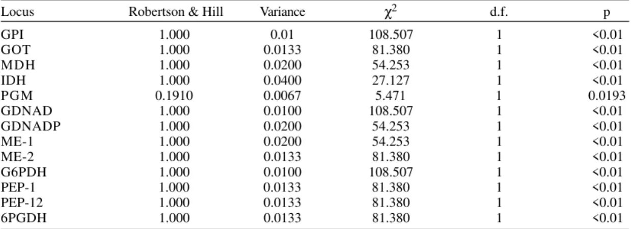
Hardy-Weinberg equilibrium - The Hardy-Weinberg equilibrium analysis showed the inexistence of this equilibrium at all levels. In this case, by using the f of Robertson and Hill (1984), an excess of homozygosis was found for the total population (f = 0.1910; χ2 = 5.471; 1 df; P <0.05; see Table II), although applying the F of Wright, a non significant excess of heterozygosis was obtained

(F = -0.3158; χ2 = 14.958, 21 df; P =0.825). Márquez

et al. (1998) found an overall observed hetero-zygosity, which was not statistically different from the Hardy-Weinberg proportions. However, the overall and the individual absence of Hardy-Weinberg equilibrium of this magnitude in our data is typical of a clonal structure.

Levels of individual diversity and hetero-geneity in the T. cruzi stocks surveyed in Colombia - In this study the proportion of different zy-modemes for Colombia is noteworthy higher (87 %) than the val-ues obtained by previous authors. However, the mean heterozygosity (H) found in this work (around H = 0.04) is substantially lower (ten times lesser) than the value reported by Márquez et al. (1998) (H = 0.40). Our value is more similar to that reported by Tibayrenc and Ayala (1988) (H = 0.06). In addition,

we found only one locus (PGM) in heterozygote

condition out of the 13 loci analyzed (7.7 %). On the contrary, Márquez et al. (1998) found heterozygous

genotypes for the loci Alat, Mpi, Pep, Gpi, Acon,

TABLE II

Hardy-Weinberg equilibrium tests using the Robertson & Hill’s f statistics of the 13 isoenzymatic loci analyzed in 23 Colombian Trypanosoma cruzi stocks

Locus Robertson & Hill Variance χ2 _d.f. _p

GPI 1.000 0.01 108.507 1 <0.01

GOT 1.000 0.0133 81.380 1 <0.01

MDH 1.000 0.0200 54.253 1 <0.01

IDH 1.000 0.0400 27.127 1 <0.01

PGM 0.1910 0.0067 5.471 1 0.0193

GDNAD 1.000 0.0100 108.507 1 <0.01

GDNADP 1.000 0.0200 54.253 1 <0.01

ME-1 1.000 0.0200 54.253 1 <0.01

ME-2 1.000 0.0133 81.380 1 <0.01

G6PDH 1.000 0.0100 108.507 1 <0.01

PEP-1 1.000 0.0133 81.380 1 <0.01

PEP-12 1.000 0.0133 81.380 1 <0.01

6PGDH 1.000 0.0133 81.380 1 <0.01

(6)

3 6 3 6 3 6 3 6

Icd, Ldh, Asat and Pgm (in lower magnitude for this locus than the value reported here) out of the13 loci analyzed (9/13 = 69. 2 %).

Our estimate of genetic heterogeneity among the T. cruzi stocks analyzed in Colombia is one of the highest reported for whatever organism in the

world (G_ST = 0.93) and it is strongly significant.

For 33 Colombian clonets, Márquez et al. (1998)

obtained a F_ST range of 0.33-0.67, also highly

significant. Therefore, there is agreement between both works in this aspect.

Genetic distances - The genetic distances found

between pairs of Colombian stocks of T. cruzi are

enormous in many cases, suggesting an extensive degree of genetic diferentiation between pairs of stocks. Tibayrenc et al. (1986b) found for Latin America values of Nei’s distances ranging from 0.017 to 2.015, with a mean value of 0.757 ± 0.478. Although the geographical span analyzed in Colombia is con-siderably smaller, the values found ranged from 0.0-0.147 to 1.833, with mean values according to those for all Latin America by Tibayrenc and Ayala (1988) (Table III). This means that the enormous divergence between the stocks studied in Colombia is of the same order of magnitude than that found by Tibayrenc and Ayala (1988) for 121 stocks covering all Latin America, including populations of USA. The results obtained applying the distance of Nei were also found using the other genetic distances

calcu-lated. The Chritidia stocks differed significantly from

those of T. cruzi with Nei’s distances of 2.545.

Re-markably, the values between pairs of stocks of T.

cruzi and Chrithidia were in some cases smaller

than those between certain pairs of stocks of T. cruzi.

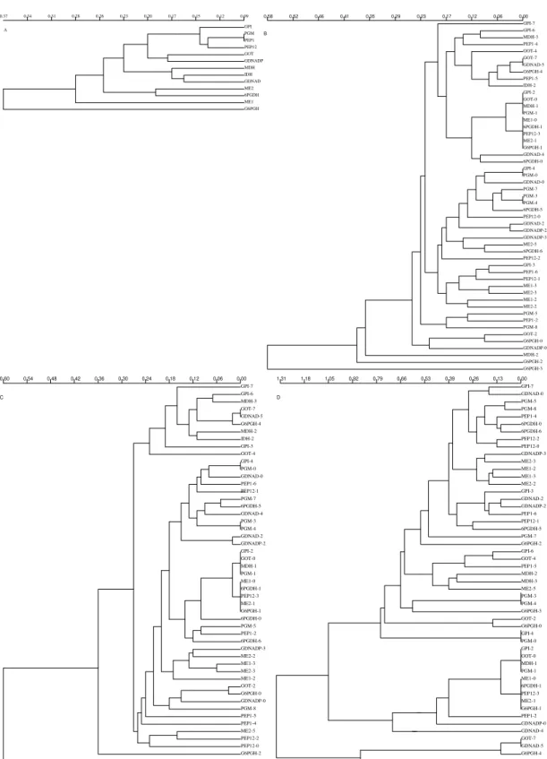
The most prominent dendrograms were ob-served when applying the algorithm WPGMA, and the distances of Prevosti and Cavalli-Sforza & Edwards. Both dendrograms (Fig. 1) clearly sepa-rated Crithidia from all T. cruzi stocks. The first T. cruzi stock which diverged was that of Chile (MN) representing the Z2 zymodeme of domestic cycle. Otherwise, the Bolivian stock (SO34) was more re-lated to the Colombian stocks, showing that these stocks basically belong to the Z1 zymodemes. In-side of the Colombian array, those of Amalfi (Antioquia) and some of the Cundinamarca depart-ment (central Colombia) were the first which di-verged. However, there is not a clearly defined number of clusters within the departments. These dendrograms highly differed from the Single analy-sis with the Nei’s distance because of grouping together stocks 5 (Arboledas, North Santander) and 7 (Zetaquirá, Boyacá) with the cluster where are stocks 1 (El Zulia, North-Santander) and 8 (Guateque, Boyacá). The dendrogram generated with the method of neighbor-joining and the dis-tance of Prevosti leads to a similar result,

display-TABLE III

E III

Nei’

s genetic distance matrix among 23 Colombian

(7)

El Zulia (Norte de Santander) Guateque (Boyacá) Sabanalarga 2 (Casanare) Ricaurte 5 (Cundinamarca)

Mariquita (Tolima) Tibú (Norte de Santander) Ricaurte 2 (Cundinamarca) Ricaurte 6 (Cundinamarca) Tibú 2 (Norte de Santander) Paratebueno (Cundinamarca)

Durania 2 (Norte de Santander) Ricaurte 4 (Cundinamarca) Durania 1 (Norte de Santander) Sabanalarga 1 (Casanare)

Catatumbo (Norte de Santander)

Ricaurte 1 (Cundinamarca) Ricaurte 3 (Cundinamarca) Choachí (Cundinamarca) Arboledas (Norte de Santander) Zetaquirá (Boyacá) Durania 3 (Norte de Santander)

Amalfi (Antioquia) Chiriguaná (Cesar)

Crithidia 1 Crithidia 2

43.14 38.82 34.51 30.20 25.88 21.57 17.25 12.94 8.63 4.31 0.00

A El Zulia (Norte de Santander)

Guateque (Boyacá) Sabanalarga 2 (Casanare) Ricaurte 5 (Cundinamarca)

Mariquita (Tolima) Tibú (Norte de Santander)

Ricaurte 2 (Cundinamarca) Ricaurte 6 (Cundinamarca) Tibú 2 (Norte de Santander)

Paratebueno (Cundinamarca) Durania 2 (Norte de Santander) Ricaurte 4 (Cundinamarca) Durania 1 (Norte de Santander) Sabanalarga 1 (Casanare)

Catatumbo (Norte de Santander Ricaurte 1 (Cundinamarca) Ricaurte 3 (Cundinamarca)

Choachí (Cundinamarca) Arboledas (Norte de Santander) Zetaquirá (Boyacá) Durania 3 (Norte de Santander) Amalfi (Antioquia)

Chiriguaná (Cesar)

1.45 1.30 1.16 1.01 0.87 0.72 0.58 0.43 0.29 0.14 0.00

B

El Zulia (Norte de Santander) Guateque (Boyacá) Sabanalarga 2 (Casanare) Ricaurte 5 (Cundinamarca)

Mariquita (Tolima)

Tibú (Norte de Santander) Ricaurte 2 (Cundinamarca)

Ricaurte 6 (Cundinamarca) Tibú 2 (Norte de Santander) Paratebueno (Cundinamarca) Durania 2 (Norte de Santander) Ricaurte 4 (Cundinamarca) Durania 1 (Norte de Santander) Sabanalarga 1 (Casanare)

Catatumbo (Norte de Santander) Ricaurte 1 (Cundinamarca) Ricaurte 3 (Cundinamarca)

Choachí (Cundinamarca) Arboledas (Norte de Santander) Zetaquirá (Boyacá) Durania 3 (Norte de Santander)

Amalfi (Antioquia) Chiriguaná (Cesar)

12.00 11.00 10.00 9.00 8.00 7.00 6.00 5.00 4.00 3.00 2.00

C

Z1 Zymodeme (Bolivia SO34)

Z2 Zymodeme (Chile MN) Z1 Zymodeme (Bolivia SO34) Z2 Zymodeme (Chile MN)

Z1 Zymodeme (Bolivia SO34)

Z2 Zymodeme (Chile MN)

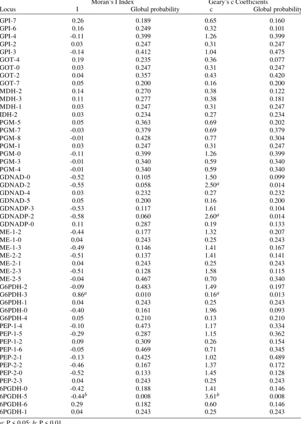
Fig. 1: dendrograms showing the genetic relationships among 23 Colombian Trypanosoma cruzi and two reference (Z2 Bolivian zymodeme and Z1 Chilean zymodeme) stocks by using 13 isoenzymatic loci. Two Chritidia stocks were used as outgroups. A: WPGMA algorithm with the Cavalli-Sforza & Edwards’s chord distance; B: single algorithm with the Nei’s genetic distance; C: neighbor-joining algorithm with the Prevosti’s distance

ing it more clearly than the other methods the group comprised by stocks 5, 6, 7 and 12.

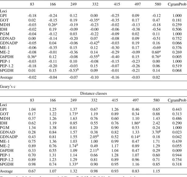
Spatial autocorrelation analysis - The interpretations based on the results derived from the spatial autocorrelation analysis, due to the use of genotypic multistates, or the use of the allelic frequencies, are remarkably different.

Genotypic multistates: by using Moran’s I

in-dex, only G6pdh out of the 13 variables studied

was significant (p = 0.005) with a clear circular clinal structure, showing a 1DC significantly positive, 4DC significantly negative, and the 5DC significantly

positive again when seven DC were used. Got

follows a similar spatial pattern, but it did not reach the level of statistical significance. Two other

markers, Gdh-Nadp+ and 6pgdh, also stood close

to the point of statistical significance, and displayed a strong decline in genetic similarity at 4DC and 3DC, respectively (Table IV). The average correlogram is clearly not significant. With the Geary’s c coefficient, the same trends are observed more clearly. G6PDH showed a significant circular cline, as with the Moran’s I index. In contrast to

(8)

dif-3 8 3 8 3 8 3 8

ferentiation at long distance (Sokal et al. 1989), with an extremely high value at 7DC (c = 3.70; p <0.0001).

Gdh-Nadp+ also displayed a significant circular cline. The remaining variables did not display any kind of spatial structure. In general, the application of genotypic multistates did not reveal the pres-ence of much significant spatial structure. This is reflected in the following results: both the percent of significant coefficients of autocorrelation, as well as the percent of significant global correlograms, did not differ from the 5% of type I error for any of the two indices applied (Moran and Geary: 8.79%;

8/91; χ2 = 1.05, 1 df, NS; Moran: 7.69%; 1/13; NS;

Geary: 23%; 3/13; NS, respectively). Neither the 13 variables analyzed showed significant values for a single autocorrelation coefficient without defining distance classes (Table V).

The analysis of similarity for the correlograms derived from the matrices of distances of Manhat-tan for the Moran’s I index is based on the percent of distances between the correlograms of pairs of variables with values smaller than 0.1. This per-centage was 1.3%, which did not even reach the error type I of 5%. By applying genotypic

TABLE IV

Spatial autocorrelation correlograms using Moran’s I and Geary’s c coefficient of the 13 isoenzimatic loci analyzed in this study with multistate unordered genotypes, and the average correlogram for seven equal distance classes

for 23 Colombian Trypanosoma cruzi stocks

Moran I index

Distance classes

83 166 249 332 415 497 580 CgramProb

Loci

GPI -0.18 -0.24 0.12 0.00 -0.25 0.09 -0.12 1.000

GOT 0.02 -0.15 0.19 -0.35a -0.35 0.17 0.47 0.181

MDH -0.03 0.26a -0.19 -0.23 -0.02 -0.13 -0.18 0.259

IDH -0.02 0.19 -0.09 -0.00 -0.06 -0.38 -0.54 0.506

PGM -0.04 -0.12 0.03 -0.22 -0.09 0.02 0.11 1.000

GDNAD 0.00 -0.14 -0.20 0.07 -0.08 0.09 -0.51 0.752

GDNADP -0.05 0.04 -0.06 -0.42b -0.03 0.19 0.16 0.066

ME-1 -0.06 -0.35 0.15 0.12 -0.30 0.17 -0.69 0.376

ME-2 -0.08 -0.01 -0.36 0.14 -0.29 -0.09 0.60a 0.269

G6PDH 0.36a 0.12 -0.08 -0.55b -0.40 0.15 0.76a 0.005

PEP-1 -0.03 -0.11 0.10 -0.08 -0.15 -0.23 0.00 1.000

PEP-1.2 -0.18 -0.20 -0.03 0.15 -0.07 -0.26 0.06 0.519

6PGDH 0.01 0.15 -0.53b 0.09 -0.01 -0.21 0.14 0.068

Average -0.02 -0.04 -0.07 -0.10 -0.16 -0.03 0.02

Geary’s c

Distance classes

83 166 249 332 415 497 580 CgramProb

Loci

GPI 1.04 1.25 1.37 0.67 1.26 0.46 0.65 0.443

GOT 0.17 1.22 1.73a _1.19 _0.89 _0.34 _0.88 _0.313

MDH 0.37 1.26 1.63 0.76 0.60 1.10 1.43 0.486

IDH 0.62 1.19 0.85 0.55 0.76 1.86a _2.42 _0.290

PGM 1.34 1.38 0.81 1.20 0.90 0.53 0.24 1.000

GDNAD 0.28 0.84 1.57 0.38 0.82 1.33 3.70b _0.023

GDNADP 0.43 0.81 1.55 2.05b _0.52 _0.14a _0.18 _0.042

ME-1 0.75 1.36 1.03 1.00 0.99 0.47 1.71 0.439

ME-2 0.89 0.76 1.74b _0.49 _1.17 _0.89 _1.29 _0.055

G6PDH 0.33 0.55 1.09 2.11b _1.04 _0.47 _0.29 _0.009

PEP-1 0.70 1.31 1.14 0.66 1.28 1.07 0.60 0.944

PEP-1.2 0.89 1.23 1.29 0.81 0.89 0.96 0.71 0.754

6PGDH 0.98 0.74 1.33a _0.90 _0.95 _1.16 _0.85 _0.318

Average 0.67 1.07 1.32 0.98 0.93 0.83 1.15

(9)

multistates, it was not possible to reveal any de-gree of similarity in the spatial distribution of the 13 variables analyzed (Fig. 2A).

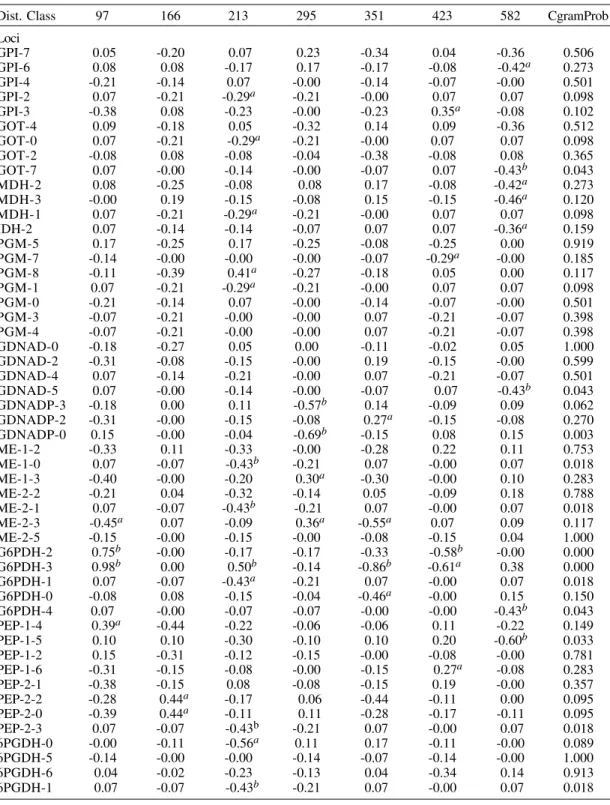
Allelic frequencies- The use of the allelic fre-quencies, in contrast, revealed a significant spatial structure of various kinds for the 51 variables ana-lyzed for the 7 and 8 DC defined. The alleles that showed significant global correlograms with the Moran’s I index and with 7 DC were 12 (12/51 = 23. 529 % of significant overall correlograms) and there was 10.9 % of significant individual autocorrelation coefficients (39/357), both percentages significant

(Table VI): Got 7, Gdnad 5, G6pdh 4 and Pep1 5

with a clear genetic differentiation at long distance;

Gdh-Nadp+0 presents a typical symmetrical circu-lar cline with 4DC being significantly negative, and

1DC and 7DC the most positive of all seen; Me1-0,

Me2-1, G6pdh-1, Pep2-3 and 6pgdh 1 with a sig-nificant global structure of regional genetic patch

from 166 to 213 km; G6pdh 2 has the structure of a

regional patch, of a considerably larger size than the other alleles with this structure (1DC signifi-cantly positive, and 6DC signifisignifi-cantly negative) and

G6pdh 3 with high genetic similarity in the first 213 km and strong genetic differences from 351 km. In addition, other nine alleles showed correlograms very near to the significance border (9/51 = 10.92%)

Gpi 2, Got 0, Mdh 1, 6pgdh 0 and Pgm 1, with a near global structure of regional genetic patch from 166 to 213 km. The high similarity between the spa-tial patterns for the frequencies of those alleles at different loci may be an important evidence of a strong linkage disequilibrium between groups of

alleles of different loci. Gnadp 3 showed a

correlogram typical of a circular cline, Pep2 2 and

Pep2 0 presented negative values for the first

dis-tance class but significant ones for the second class distance (97-166 km). With 8 DC defined the results were similar. In fact, the spatial genetic structure is larger and highly significant, as well. For the Moran I index, 31.4% (16/51) of the overall correlograms and 10.5% (43/408) of the individual autocorrelation coefficients were respectively significant. The alle-les which showed significant correlograms were

Gpi 2, Gpi 3, Got 0, Got 7, Mdh 1, Pgm 1, Gdnad 5, Gnadp 0, Me1 0, Me2 1, G6pdh 2, G6pdh 3, G6pdh 1, G6pdh 4 Pep2 3 and 6Pgdh 1. The vast majority was significant with 7 DC defined, or was significant borderline, as well.

Applying the Geary’s c coefficient, the situation was similar. With 7 DC defined, 27.4% of significant overall correlograms (14/51) and 15.4% of signifi-cant individual autocorrelation coefficients (55/357):

Got 7, Gdnad 5, G6pdh 4 and Pep1 5 showed

sig-nificant differentiation at long distance; Gdnadp 3,

Gdnadp 0 and G6pdh 0 yielded circular clines; Me1 0, Me2 1, G6pdh 1, Pep1 2 Pep2 3 and 6pgdh 1

showed significant regional patches; G6pdh 3

showed striking genetic similarity until 213 km and a strong disimilarity between the stocks at 351 km, and G6pdh 2 showed a monotonic clinal divergence until 423 km, with the last DC not significant. Addi-tionally, 13.7% of other correlograms were

border-line significant (7/51; Gp1 2, Got 0, Mdh 2, Mdh 1,

Pgm 5, Pgm 1 and G6pdh 0). With 8 DC, 33.3% (17/ 51) of overall correlograms and 12.5% (51/408) of individual autocorrelation coefficients were signifi-cant, respectively. The alleles showing significant

correlograms were Gp1 2, Got 0, Got 2, Got 7, Mdh

1, Pgm 1, Gdnad 5, Gdnadp 0, Me1 0, Me2 1, 6pgdh 3, G6pdh 1, G6pdh 4, Pep1 5, Pep1 2, Pep2 3 and

6Pgdh 1. The spatial trends found were very similar

TABLE V

Single autocorrelation coefficients for each one of the 13 isoenzymatic loci analyzed in 23 Colombian

Trypanosoma cruzi stocks considering unordered multistate genotypes. The point pairs were weighted as the

inverse square separation distance between the stocks

Coefficients Moran’s I Index Geary’s c

Locus I Global probability c Global probability

GPI 0.09 0.328 0.72 0.289

GOT 0.03 0.381 0.32 0.142

MDH 0.03 0.372 0.34 0.151

IDH 0.11 0.277 0.38 0.181

PGM -0.02 0.432 0.90 0.436

GDNAD -0.15 0.403 0.55 0.243

GDNADP -0.21 0.337 0.74 0.322

ME-1 -0.16 0.398 0.93 0.445

ME-2 -0.27 0.291 0.94 0.452

G6PDH 0.35 0.114 0.80 0.344

PEP-1 -0.08 0.485 0.67 0.242

PEP-1.2 -0.41 0.182 1.22 0.291

(10)

4 0 4 0 4 0 4 0

GPI PGM PEP12 PEP1 GOT GDNADP MDH IDH GDNAD ME2 6PGDH ME1 G6PGH

0.37 0.34 0.31 0.28 0.26 0.23 0.20 0.17 0.15 0.12 0.09

A

Fig. 2-A: UPGMA analysis of the spatial autocorrelation coefficients with the Moran’s I index of the 13 isoenzymatic loci analyzed in this study, considering genotypic unordered multistates having defined seven distance classes with constant geo-graphical sizes; B: UPGMA analysis of the spatial autocorrelation coefficients with the Moran’s I index of the 51 alleles analyzed in this study, considering allele frequencies, having defined six distance classes with a relatively equal number of point pairs per distance class; C: UPGMA analysis of the spatial autocorrelation coefficients with the Moran’s I index of the 51 alleles analyzed in this study, considering allele frequencies, having defined seven distance classes with a relatively equal number of point pairs per distance class; D: UPGMA analysis of the spatial autocorrelation coefficients with the Moran’s I index of the 51 alleles analyzed in this study, considering allele frequencies, having defined eight distance classes with constant geographical sizes.

GPI-7 GPI-6 IDH-2 PGM-5 PGM-7 PGM-8 PGM-1 PGM-0 PGM-3 PGM-4 GDNADP-0 GDNADP-2 GDNAD-4 GDNAD-5 GDNADP-3 GDNAD-2 GDNAD-0 ME1-2 ME1-0 ME1-3 ME2-2 ME2-1 ME2-3 ME2-5 G6PGH-2 G6PGH-3 G6PGH-1 G6PGH-0 G6PGH-4 PEP1-4 PEP1-5 PEP1-2 PEP1-6 PEP12-1 PEP12-2 PEP12-0 PEP12-3 6PGDH-0 6PGDH-5 6PGDH-6 6PGDH-1 MDH-3 GOT-4 GOT-7 GPI-2 GOT-0 MDH-1 GPI-4 GPI-3 GOT-2 MDH-2 1.31 1.18 1.05 0.92 0.79 0.66 0.53 0.39 0.26 0.13 0.00

D GPI-7 GPI-6 IDH-2 PGM-5 PGM-7 PGM-8 PGM-1 PGM-0 PGM-3 PGM-4 GDNADP-0 GDNADP-2 GDNAD-4 GDNAD-5 GDNADP-3 GDNAD-2 GDNAD-0 ME1-2 ME1-0 ME1-3 ME2-2 ME2-1 ME2-3 ME2-5 G6PGH-2 G6PGH-3 G6PGH-1 G6PGH-0 G6PGH-4 PEP1-4 PEP1-5 PEP1-2 PEP1-6 PEP12-1 PEP12-2 PEP12-0 PEP12-3 6PGDH-0 6PGDH-5 6PGDH-6 6PGDH-1 MDH-3 GOT-4 GOT-7 GPI-2 GOT-0 MDH-1 GPI-4 GPI-3 GOT-2 MDH-2 0.58 0.52 0.46 0.41 0.35 0.29 0.23 0.17 0.12 0.06 0.00

B GPI-7 GPI-6 IDH-2 PGM-5 PGM-7 PGM-8 PGM-1 PGM-0 PGM-3 PGM-4 GDNADP-0 GDNADP-2 GDNAD-4 GDNAD-5 GDNADP-3 GDNAD-2 GDNAD-0 ME1-2 ME1-0 ME1-3 ME2-2 ME2-1 ME2-3 ME2-5 G6PGH-2 G6PGH-3 G6PGH-1 G6PGH-0 G6PGH-4 PEP1-4 PEP1-5 PEP1-2 PEP1-6 PEP12-1 PEP12-2 PEP12-0 PEP12-3 6PGDH-0 6PGDH-5 6PGDH-6 6PGDH-1 MDH-3 GOT-4 GOT-7 GPI-2 GOT-0 MDH-1 GPI-4 GPI-3 GOT-2 MDH-2 0.60 0.54 0.48 0.42 0.36 0.30 0.24 0.18 0.12 0.06 0.00

(11)

TABLE VI

Spatial autocorrelation correlograms using Moran’s I index and Geary’s c coefficient of the 51 allele frequencies from 13 isoenzymatic loci analyzed in this study (A) for seven unequal distance classes and (B) for eight constant

distance classes for 23 Colombian Trypanosoma cruzi stocks. Distance classes in kilometers (A)

Moran I index

Distance classes

Dist. Class 97 166 213 295 351 423 582 CgramProb

Loci

GPI-7 0.05 -0.20 0.07 0.23 -0.34 0.04 -0.36 0.506

GPI-6 0.08 0.08 -0.17 0.17 -0.17 -0.08 -0.42a _0.273

GPI-4 -0.21 -0.14 0.07 -0.00 -0.14 -0.07 -0.00 0.501

GPI-2 0.07 -0.21 -0.29a -0.21 -0.00 0.07 0.07 0.098

GPI-3 -0.38 0.08 -0.23 -0.00 -0.23 0.35a -0.08 0.102

GOT-4 0.09 -0.18 0.05 -0.32 0.14 0.09 -0.36 0.512

GOT-0 0.07 -0.21 -0.29a -0.21 -0.00 0.07 0.07 0.098

GOT-2 -0.08 0.08 -0.08 -0.04 -0.38 -0.08 0.08 0.365

GOT-7 0.07 -0.00 -0.14 -0.00 -0.07 0.07 -0.43b _0.043

MDH-2 0.08 -0.25 -0.08 0.08 0.17 -0.08 -0.42a 0.273

MDH-3 -0.00 0.19 -0.15 -0.08 0.15 -0.15 -0.46a 0.120

MDH-1 0.07 -0.21 -0.29a _-0.21 _-0.00 _0.07 _0.07 _0.098

IDH-2 0.07 -0.14 -0.14 -0.07 0.07 0.07 -0.36a 0.159

PGM-5 0.17 -0.25 0.17 -0.25 -0.08 -0.25 0.00 0.919

PGM-7 -0.14 -0.00 -0.00 -0.00 -0.07 -0.29a -0.00 0.185

PGM-8 -0.11 -0.39 0.41a _-0.27 _-0.18 _0.05 _0.00 _0.117

PGM-1 0.07 -0.21 -0.29a -0.21 -0.00 0.07 0.07 0.098

PGM-0 -0.21 -0.14 0.07 -0.00 -0.14 -0.07 -0.00 0.501

PGM-3 -0.07 -0.21 -0.00 -0.00 0.07 -0.21 -0.07 0.398

PGM-4 -0.07 -0.21 -0.00 -0.00 0.07 -0.21 -0.07 0.398

GDNAD-0 -0.18 -0.27 0.05 0.00 -0.11 -0.02 0.05 1.000

GDNAD-2 -0.31 -0.08 -0.15 -0.00 0.19 -0.15 -0.00 0.599

GDNAD-4 0.07 -0.14 -0.21 -0.00 0.07 -0.21 -0.07 0.501

GDNAD-5 0.07 -0.00 -0.14 -0.00 -0.07 0.07 -0.43b 0.043

GDNADP-3 -0.18 0.00 0.11 -0.57b _0.14 _-0.09 _0.09 _0.062

GDNADP-2 -0.31 -0.00 -0.15 -0.08 0.27a _-0.15 _-0.08 _0.270

GDNADP-0 0.15 -0.00 -0.04 -0.69b -0.15 0.08 0.15 0.003

ME-1-2 -0.33 0.11 -0.33 -0.00 -0.28 0.22 0.11 0.753

ME-1-0 0.07 -0.07 -0.43b _-0.21 _0.07 _-0.00 _0.07 _0.018

ME-1-3 -0.40 -0.00 -0.20 0.30a -0.30 -0.00 0.10 0.283

ME-2-2 -0.21 0.04 -0.32 -0.14 0.05 -0.09 0.18 0.788

ME-2-1 0.07 -0.07 -0.43b _-0.21 _0.07 _-0.00 _0.07 _0.018

ME-2-3 -0.45a _0.07 _-0.09 _0.36a _-0.55a _0.07 _0.09 _0.117

ME-2-5 -0.15 -0.00 -0.15 -0.00 -0.08 -0.15 0.04 1.000

G6PDH-2 0.75b -0.00 -0.17 -0.17 -0.33 -0.58b -0.00 0.000

G6PDH-3 0.98b _0.00 _0.50b _-0.14 _-0.86b _-0.61a _0.38 _0.000

G6PDH-1 0.07 -0.07 -0.43a -0.21 0.07 -0.00 0.07 0.018

G6PDH-0 -0.08 0.08 -0.15 -0.04 -0.46a -0.00 0.15 0.150

G6PDH-4 0.07 -0.00 -0.07 -0.07 -0.00 -0.00 -0.43b _0.043

PEP-1-4 0.39a -0.44 -0.22 -0.06 -0.06 0.11 -0.22 0.149

PEP-1-5 0.10 0.10 -0.30 -0.10 0.10 0.20 -0.60b 0.033

PEP-1-2 0.15 -0.31 -0.12 -0.15 -0.00 -0.08 -0.00 0.781

PEP-1-6 -0.31 -0.15 -0.08 -0.00 -0.15 0.27a -0.08 0.283

PEP-2-1 -0.38 -0.15 0.08 -0.08 -0.15 0.19 -0.00 0.357

PEP-2-2 -0.28 0.44a -0.17 0.06 -0.44 -0.11 0.00 0.095

PEP-2-0 -0.39 0.44a _-0.11 _0.11 _-0.28 _-0.17 _-0.11 _0.095

PEP-2-3 0.07 -0.07 -0.43b -0.21 0.07 -0.00 0.07 0.018

6PGDH-0 -0.00 -0.11 -0.56a 0.11 0.17 -0.11 -0.00 0.089

6PGDH-5 -0.14 -0.00 -0.00 -0.14 -0.07 -0.14 -0.00 1.000

6PGDH-6 0.04 -0.02 -0.23 -0.13 0.04 -0.34 0.14 0.913

6PGDH-1 0.07 -0.07 -0.43b _-0.21 _0.07 _-0.00 _0.07 _0.018

(12)

4 2 4 2 4 2 4 2

Geary’s c

Distance classes

Dist. Class 97 166 213 295 351 423 582 CgramProb

Loci

GPI-7 0.88 1.13 0.88 0.75 1.25 0.88 1.25 0.708

GPI-6 0.39 0.97 0.97 1.36 0.97 0.78 1.56 0.372

GPI-4 2.00 1.50 0.00 0.50 1.50 1.00 0.50 0.501

GPI-2 0.00 2.00 2.50a _2.00 _0.50 _0.00 _0.00 _0.098

GPI-3 1.88a 0.27a 1.35 0.54 1.35 0.81 0.81 0.262

GOT-4 0.48a _0.95 _1.11 _1.75a _0.95 _0.48a _1.27 _0.115

GOT-0 0.00 2.00 2.50a 2.00 0.50 0.00 0.00 0.098

GOT-2 0.81 0.27a _0.81 _2.15a _1.88a _0.81 _0.27 _0.233

GOT-7 0.00 0.50 1.50 0.50 1.00 0.00 3.50b 0.043

MDH-2 0.39 1.75a _1.36 _0.97 _0.19a _0.78 _1.56 _0.094

MDH-3 0.54 1.35 1.08 0.81 0.00a 1.08 2.15a 0.136

MDH-1 0.00 2.00 2.50a _2.00 _0.50 _0.00 _0.00 _0.098

IDH-2 0.00 1.50 1.50 1.00 0.00 0.00 3.00a 0.159

PGM-5 0.78 1.75a _0.78 _1.17 _0.78 _1.17 _0.58 _0.094

PGM-7 1.50 0.50 0.50 0.50 1.00 2.50a 0.50 0.185

PGM-8 1.11 1.59a _0.48a _1.11 _0.95 _1.11 _0.64 _0.136

PGM-1 0.00 2.00 2.50a 2.00 0.50 0.00 0.00 0.098

PGM-0 2.00 1.50 0.00 0.50 1.50 1.00 0.50 0.501

PGM-3 1.00 2.00 0.50 0.50 0.00 2.00 1.00 0.398

PGM-4 1.00 2.00 0.50 0.50 0.00 2.00 1.00 0.398

GDNAD-0 0.95 1.11 1.11 0.64 1.11 0.95 1.11 1.000

GDNAD-2 1.62 0.81 1.08 0.54 1.35 1.08 0.54 0.754

GDNAD-4 0.00 1.50 2.00 0.50 0.00 2.00 1.00 0.501

GDNAD-5 0.00 0.50 1.50 0.50 1.00 0.00 3.50b _0.043

GDNADP-3 0.95 0.64 1.27 1.91b 0.95 0.80 0.48 0.025

GDNADP-2 1.62 0.54 1.08 0.81 1.08 1.08 0.81 0.794

GDNADP-0 0.00a 0.54 2.15a 2.96b 1.08 0.27a 0.00 0.003

ME-1-2 1.17 0.78 1.30 1.17 1.17 0.65 0.78 0.459

ME-1-0 0.00 1.00 3.50b 2.00 0.00 0.50 0.00 0.018

ME-1-3 1.26 0.84 0.98 0.98 1.26 0.84 0.84 1.000

ME-2-2 1.13 0.88 1.25 1.13 0.88 1.00 0.75 0.708

ME-2-1 0.00 1.00 3.50b _2.00 _0.00 _0.50 _0.00 _0.018

ME-2-3 1.43 0.80 0.80 1.11 1.59a 0.80 0.48 0.178

ME-2-5 1.08 0.54 1.08 0.54 0.81 1.08 1.88 0.582

G6PDH-2 0.58 0.58 0.97 0.97 1.36 1.94b 0.58 0.019

G6PDH-3 0.00b _0.88 _0.50b _1.13 _1.75b _1.50a _1.25 _0.000

G6PDH-1 0.00 1.00 3.50b 2.00 0.00 0.50 0.00 0.018

G6PDH-0 0.81 0.27 1.08 2.15a _2.15b _0.54 _0.00 _0.060

G6PDH-4 0.00 0.50 1.00 1.00 0.50 0.50 3.50b 0.043

PEP-1-4 0.78 1.30 1.04 0.91 1.04 0.91 1.04 0.706

PEP-1-5 0.56a 0.84 1.12 1.26 0.84 0.56a 1.82b 0.011

PEP-1-2 0.00a _1.62 _2.42b _1.08 _0.54 _0.81 _0.54 _0.048

PEP-1-6 1.62 1.08 0.81 0.54 1.08 1.08 0.81 0.794

PEP-2-1 1.88a _1.08 _0.27 _0.81 _1.08 _0.35 _0.54 _0.288

PEP-2-2 1.17 0.52a 1.04 0.78 1.30 1.04 1.17 0.133

PEP-2-0 1.30 0.52a _1.04 _0.91 _1.30 _1.04 _0.91 _0.133

PEP-2-3 0.00 1.00 3.50b 2.00 0.00 0.50 0.00 0.018

6PGDH-0 1.04 0.91 1.43a _0.91 _0.91 _1.04 _0.78 _0.213

6PGDH-5 1.50 0.50 0.50 1.50 1.00 1.50 0.50 1.000

6PGDH-6 0.88 1.00 1.13 1.00 0.88 1.25 0.88 0.922

(13)

(B)

Moran I index

Distance classes

Dist. Class 73 145 218 290 363 435 508 580 CgramProb

Loci

GPI-7 0.07 -0.16 0.02 0.18 -0.18 -0.02 -0.04 -1.00a _0.178

GPI-6 0.14 0.07 -0.13 -0.48a _0.31a _-0.27 _-0.25 _-0.69 _0.103

GPI-4 -0.22 -0.01 -0.09 -0.02 -0.12 -0.02 -0.04 0.07 0.967

GPI-2 0.07 -0.01 -0.36b -0.29 0.02 0.07 0.07 0.07 0.019

GPI-3 -0.37 -0.09 -0.13 0.06 -0.21 0.49b -0.08 -0.13 0.045

GOT-4 0.12 -0.03 -0.08 -0.15 -0.04 0.14 -0.32 -0.66 0.751

GOT-0 0.07 -0.01 -0.36b _-0.29 _0.02 _0.07 _0.07 _0.07 _0.019

GOT-2 -0.06 -0.01 -0.02 0.20 -0.42a -0.04 0.04 0.15 0.086

GOT-7 0.07 -0.01 -0.09 -0.02 -0.03 0.07 -0.36b -0.73b 0.021

MDH-2 0.14 -0.02 -0.25 0.25 0.08 -0.27 -0.25 -0.69 0.605

MDH-3 0.05 0.20 -0.13 0.06 0.05 -0.33 -0.31 -0.71 0.407

MDH-1 0.07 -0.01 -0.36b _-0.29 _0.02 _0.07 _0.07 _0.07 _0.019

IDH-2 0.07 -0.08 -0.14 -0.02 0.02 -0.02 -0.25 -0.46b 0.389

PGM-5 -0.20 0.07 0.12 -0.27 -0.09 -0.27 0.00 -0.06 1.000

PGM-7 -0.12 -0.08 0.02 -0.02 -0.12 -0.20 -0.04 0.07 0.883

PGM-8 -0.38 -0.15 0.24a _-0.32 _-0.02 _-0.12 _-0.05 _0.02 _0.325

PGM-1 0.07 -0.01 -0.36b _-0.29 _0.02 _0.07 _0.07 _0.07 _0.019

PGM-0 -0.22 -0.01 -0.09 -0.02 -0.12 -0.02 -0.04 0.07 0.967

PGM-3 -0.03 -0.31a 0.02 0.07 0.02 -0.29a -0.04 -0.20 0.104 PGM-4 -0.03 -0.31a 0.02 0.07 0.02 -0.29a -0.04 -0.20 0.104

GDNAD-0 -0.38 -0.12 -0.01 -0.09 -0.15 0.22 0.30 -0.66 0.751

GDNAD-2 -0.48a _-0.01 _-0.13 _-0.04 _0.13 _-0.13 _-0.08 _0.15 _0.313

GDNAD-4 0.07 -0.08 -0.20 -0.02 -0.03 -0.11 -0.14 0.07 0.864

GDNAD-5 0.07 -0.01 -0.09 -0.02 -0.03 0.07 0.36b -0.73b 0.021

GDNADP-3 -0.32 0.11 -0.12 -0.49 -0.08 0.07 0.36 0.09 0.451

GDNADP-2 -0.42 0.01 -0.11 -0.08 0.07 -0.09 0.15 -0.08 0.426

GDNADP-0 0.15 0.08 -0.19 -0.77b _-0.13 _0.15 _0.15 _0.15 _0.012

ME-1-2 -0.31 0.15 -0.20 -0.25 -0.00 0.13 -0.03 -0.17 1.000

ME-1-0 0.07 0.00 -0.42b -0.14 0.02 0.07 0.07 0.07 0.007

ME-1-3 -0.38 -0.06 -0.05 0.20 -0.18 0.07 0.00 -0.10 0.938

ME-2-2 -0.35 0.22 -0.25 -0.36 0.18 -0.04 -0.33 0.23 0.788

ME-2-1 0.07 0.00 -0.42b _-0.14 _0.02 _0.07 _0.07 _0.07 _0.007

ME-2-3 -0.43 0.00 -0.02 0.40a -0.32 0.05 -0.09 0.09 0.298

ME-2-5 -0.13 -0.06 -0.16 0.15 -0.13 -0.01 -0.62a 0.73b 0.079 G6PDH-2 0.56b 0.25 -0.15 -0.13 -0.44a -0.46a 0.04 0.25 0.033 G6PDH-3 0.99b _0.19 _0.50b _-0.57a _-0.79b _-0.46 _-0.38 _-0.63 _0.000

G6PDH-1 0.07 0.00 -0.42b _-0.14 _0.02 _0.07 _0.07 _0.07 _0.007

G6PDH-0 -0.13 0.08 0.18a -0.65b -0.31 -0.01 0.15 0.15 0.054 G6PDH-4 0.07 0.00 -0.12 0.07 -0.04 0.07 -0.46b -0.79b 0.008 PEP-1-4 0.39a -0.22 -0.24 -0.08 0.17 -0.23 -0.44 -0.00 0.298 PEP-1-5 0.12 0.03 0.02 -0.55a _0.13 _-0.14 _-1.00b _0.20 _0.068

PEP-1-2 0.15 -0.13 -0.24 -0.08 -0.08 -0.01 -0.04 0.15 1.000

PEP-1-6 -0.23 -0.28 -0.06 0.04 -0.08 0.20 -0.04 -0.08 0.749

PEP-2-1 -0.42 -0.13 -0.00 -0.08 0.18 -0.18 -0.23 0.15 0.426

PEP-2-2 -0.10 0.15 0.06 -0.17 -0.29 -0.11 -0.58 0.50 0.601

PEP-2-0 -0.38 0.20 0.06 0.08 -0.21 -0.23 -0.17 -0.00 0.936

PEP-2-3 0.07 0.00 -0.42b _-0.14 _0.02 _0.07 _0.07 _0.07 _0.007

6PGDH-0 -0.10 -0.01 0.36a 0.08 0.17 -0.11 -0.17 -0.00 0.340

6PGDH-5 -0.20 0.00 -0.03 -0.14 -0.14 -0.08 0.07 0.07 1.000

6PGDH-6 -0.04 0.17 -0.31 -0.06 -0.04 -0.25 0.07 0.29 0.629

(14)

4 4 4 4 4 4 4 4

Geary’s c

Distance classes

Dist. Class 73 145 218 290 363 435 508 580 CgramProb

Loci

GPI-7 0.85 1.07 0.94 0.78 1.11 0.94 0.94 1.88a _0.179

GPI-6 0.27 1.04 0.88 1.70 0.66 1.22 1.17 2.19 0.409

GPI-4 2.05 0.54 1.13 0.63 1.36 0.63 0.75 0.00 0.967

GPI-2 0.00 0.54 3.00b 2.50 0.34 0.00 0.00 0.00 0.019

GPI-3 1.84 0.87 1.01 0.34 1.28 0.67 0.81 1.01 0.626

GOT-4 0.43 0.68 1.19 1.59 1.08 0.40a 1.19 1.79 0.253

GOT-0 0.00 0.54 3.00b _2.50 _0.34 _0.00 _0.00 _0.00 _0.019

GOT-2 0.73 0.58 0.61 1.68 2.02b 0.67 0.40 0.00 0.031

GOT-7 0.00 0.54 1.13 0.63 0.68 0.00 3.00b _5.63b _0.021

MDH-2 0.27 1.25 1.60a 0.73 0.40a 1.22 1.17 2.19 0.160

MDH-3 0.37 1.44 1.01 0.34 0.37a _1.68 _1.62 _3.03a _0.245

MDH-1 0.00 0.54 3.00b 2.50 0.34 0.00 0.00 0.00 0.019

IDH-2 0.00 1.07 1.50 0.63 0.34 0.63 2.25 3.75a _0.389

PGM-5 1.06 1.04 1.17 1.22 0.80 1.22 0.58 0.73 1.000

PGM-7 1.36 1.07 0.38 0.63 1.36 1.88 0.75 0.00 0.883

PGM-8 1.30 1.19 0.84 1.19 0.87 1.19 0.72 0.60 1.000

PGM-1 0.00 0.54 3.00b _2.50 _0.34 _0.00 _0.00 _0.00 _0.019

PGM-0 2.05 0.54 1.13 0.63 1.36 0.63 0.75 0.00 0.967

PGM-3 0.68 2.68a _0.38 _0.00 _0.34 _2.50a _0.75 _1.88 _0.104

PGM-4 0.68 2.68a 0.38 0.00 0.34 2.50a 0.75 1.88 0.104

GDNAD-0 1.30 0.85 1.07 0.80 1.08 0.60 0.95 1.79 0.855

GDNAD-2 2.20a 0.58 1.01 0.67 1.10 1.01 0.81 0.00 0.166

GDNAD-4 0.00 1.07 1.88 0.63 0.68 1.25 1.50 0.00 0.864

GDNAD-5 0.00 0.54 1.13 0.63 0.68 0.00 3.00b 5.63b 0.021

GDNADP-3 1.19 0.45a _1.41 _1.91a _1.19 _0.51 _0.00a _0.48 _0.129

GDNADP-2 2.02a 0.50 0.92 0.81 1.41 0.87 0.00 0.81 0.310

GDNADP-0 0.00a _0.25a _2.20b _3.23b _1.01 _0.00a _0.00 _0.00 _0.011

ME-1-2 1.13 0.73 1.24 1.36 0.88 0.69 0.97 1.17 0.734

ME-1-0 0.00 0.47 3.41b _1.50 _0.38 _0.00 _0.00 _0.00 _0.007

ME-1-3 1.23 0.92 0.95 1.05 1.05 0.75 1.05 1.26 1.000

ME-2-2 1.25 0.70 1.19 1.31 0.75 0.94 1.25 0.75 0.659

ME-2-1 0.00 0.47 3.41b 1.50 0.38 0.00 0.00 0.00 0.007

ME-2-3 1.39 0.89 0.87 1.19 1.19 0.85 0.80 0.48 1.000

ME-2-5 1.01 0.76 1.10 0.00 1.01 0.58 2.69b 2.42 0.067

G6PDH-2 0.73 0.55 0.93 0.88 1.60a _1.67a _0.49 _0.00 _0.174

G6PDH-3 0.00b 0.70 0.51b 1.50a 1.69b 1.34 1.25 1.50 0.000

G6PDH-1 0.00 0.47 3.41b _1.50 _0.38 _0.00 _0.00 _0.00 _0.007

G6PDH-0 1.01 0.25a 0.92 2.83b 1.62 0.58 0.00 0.00 0.055

G6PDH-4 0.00 0.47 1.36 0.00 0.75 0.00 3.75b _6.00b _0.008

PEP-1-4 0.81 1.09 1.06 0.97 0.88 1.11 1.30 0.78 1.000

PEP-1-5 0.53 0.92 0.86 1.68a _0.74 _1.05 _2.10b _1.26 _0.035

PEP-1-2 0.00a 1.01 2.39b 0.81 0.81 0.58 0.67 0.00 0.020

PEP-1-6 1.35 1.51 0.73 0.40 0.81 1.44 0.67 0.81 0.924

PEP-2-1 2.02a 1.01 0.55 0.81 1.01 1.15 1.35 0.00 0.310

PEP-2-2 0.97 0.85 0.80 0.97 1.17 1.11 1.62 0.78 0.434

PEP-2-0 1.30 0.73 0.88 0.97 1.17 1.11 0.97 0.78 0.906

PEP-2-3 0.00 0.47 3.41b _1.50 _0.38 _0.00 _0.00 _0.00 _0.007

6PGDH-0 1.13 0.85 1.24 0.97 0.88 0.97 0.97 0.78 0.734

6PGDH-5 1.88 0.47 0.68 1.50 1.50 1.07 0.00 0.00 1.000

6PGDH-6 0.94 0.82 1.19 0.94 0.94 1.21 0.94 0.75 0.880

6PGDH-1 0.00 0.47 3.41b 1.50 0.38 0.00 0.00 0.00 0.007

(15)

to those obtained with the Moran’s I index and with 7 DC. On the contrary, when only 6 DC were consid-ered, with this coefficient, some spatial significant

structures changed. Pgm 5 and Pep-1 5 showed

significant global correlograms as regional patches, and differentiation at long distance, respectively. Fur-thermore, with 6 DC, 13 alleles showed significant global correlograms, and 19 alleles showed a ten-dency to spatial arrangements of no statistical sig-nificance.

There seems to be a slightly better chance to reveal spatial structures, or trends, with the use of the coefficient c of Geary than with the I of Moran. For instance, with 6 DC some of the alleles which were not detected with the Moran’s I index were

Got 4 (high similarity among neighbor stocks), Got

7 (differentiation at long distance), Got 0 (regional

patch), Got 2 (circular cline), Pgm 8 (regional patch) and Gdh-Nadp+ 3 (circular cline). It is interesting

to note that each allele of the Got locus yielded a

different spatial trend. The arrays of alleles that presented strong linkage in their spatial structures were basically the same by using the Moran’s I index and the Geary’s c coefficient, and were the same independently of 6, 7 or 8 DC chosen. When no distance classes were considered, the individual autocorrelation coefficient for each allele consisted in 105 pair comparisons. For the Moran’s I Index,

the alleles Gdnad 2 (P = 0.048), Gdnadp 2 (P =

0.05), G6pdh 3 (P = 0.01) and 6Pgdh 5 (P = 0.008)

were significant. This means that these were the alleles which displayed more significant spatial structures. For the Geary’s c coefficient, the alle-les Gdnad 2 (P = 0.014), Gdnadp 2 (P = 0.014),

G6pdh 3 (P = 0.013) and 6Pgdh 5 (P = 0.008) were also significant (Table VII). Altogether, it can be stated that the amount of spatial structure found in

Colombia for T. cruzi is noteworthy significant.

Some of the overall results support this view. The percentage of significant coefficients of autocorrelation was superior to the error type I of 5%, both for the Moran’s I and for the c of Geary for 6 DC (17.3%; 53/306; χ2 = 23.4; 1 df; P <0.001), for 7 DC (Moran: 10.9%; Geary: 15.4%) and for 8 DC (Moran: 10.5%; Geary: 12.5%). A percent value above the error type I of 5% was also found for both indices related with the number of significant global correlograms for 6 DC (Moran: 23.5%; 12/ 51; χ2 = 7.2; 1 df; P <0.01; Geary: 25.5%; 13/51; χ2 = 8.3; 1 df; P <0.01), for 7 DC (Moran: 23.5%; Geary: 27.4%) and for 8 DC (Moran: 31.4%; Geary: 33.3%). Therefore, there is not doubt about the striking

spatial structure among the Colombian T. cruzi

stocks, when the allele frequencies are employed. It is of upmost importance to determine whether it is better to obtain the spatial autocorrelation by using the allelic frequencies or the genotypic multistates. We find the use of the allelic frequencies

much more informative than that of genotypic states, since for the latter we have assigned the value of each state randomly, while ignoring the type of order and evolutionary transition that might have existed between the different genotypes. In contrast, with the results obtained when using the genotypic multistates, the analysis of correlogram similarity based on the allelic frequencies showed significant percent values of Manhattan distances. For instance, for the Moran’s I Index, a percent of Manhattan distances smaller than 0.1 of 8.8% (113/ 1275) was obtained for 6 DC and 8.4% (107/1275) for 7 DC, being both significantly superior to the error type I of 5% (χ2 = 14.6; 1 df; P < 0.001 and χ2 = 11.7; 1 df; P < 0.01). There is, therefore, a signifi-cant fraction of variables with the same patterns of spatial arrangement. For 6 DC, and with the Moran’s I coefficient, there was the presence of ten clusters

of highly spatial related alleles (Fig. 2b): (1) Gpi 6

and Mdh 3; (2) Got 4, Got 7, Gdh-Nad+ 5, G6pdh 4, Pep-1 5 and Idh 2. This array was comprised by the variables that have spatial structure of differ-entiation at long distance. Except in a few cases, it was observed that most spatial clusters contained alleles from different loci, a manifestation of

link-age disequilibrium; (3) Gpi 2, Got 0, Mdh 1, Pgm 1,

Me-1 0, Me-2 1, 6pgdh 1, Pep-2 3, Gdh-Nad+ 4

and 6pgdh 0. These were the alleles which typi-cally showed correlograms describing regional

patches: (4) Gpi 4, Pgm 0, Gdh-Nad+ 0, Pgm 7,

Pgm 3, Pgm 4, 6pgdh 5, and Pep-2 0; (5) Gdh-Nad+ 2 and Gdh-Nadp+ 2; (6) Me-2 and 6pgdh 6; (7) Gpi 3, Pep-1 6, Pep-2 1, Me-1 3 and Me-2 3; (8)

Me-1 2 and Me-2 2; (9) Pgm 5 and Pep-1 2 ; and

(10) Got 2 and G6pdh 0.

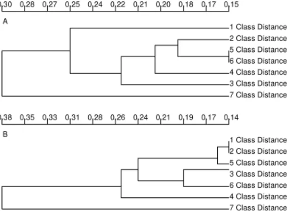
When 7 DC were used, eight clusters of highly spatial-related alleles were conformed with the Moran’s I Index and nine with the Geary´s c coef-ficient. Some of these allele-spatial related clus-ters were slightly different among them (Fig. 2C,D). In addition, we studied the similarity among the various distance classes to understand the contri-bution of each one to the spatial behaviour of the genotypes and allele frequencies studied (Fig. 3). For the analysis with 7DC, the most divergent dis-tance class, simultaneously for genotypes and for allele frequencies, was the 7 DC. Therefore, this is the distance class with the most differentiated spa-tial behaviour, which is in agreement with certain isolation-by-distance structure.

DISCUSSION

Some of the results of the population genetics analysis presented here support the point of view

of a clonal structure of the Colombian T. cruzi stocks

(16)

4 6 4 6 4 6 4 6

TABLE VII

Single autocorrelation coefficients for each one of the 51 isoenzymatic alleles analyzed in 23 Colombian

Trypanosoma cruzi stocks considering the allele frequencies. The point pairs were weighted as the inverse square

separation distance between the stocks

Moran’s I Index Geary’s c Coefficients

Locus I Global probability c Global probability

GPI-7 0.26 0.189 0.65 0.160

GPI-6 0.16 0.249 0.32 0.101

GPI-4 -0.11 0.399 1.26 0.399

GPI-2 0.03 0.247 0.31 0.247

GPI-3 -0.14 0.412 1.04 0.475

GOT-4 0.19 0.235 0.36 0.077

GOT-0 0.03 0.247 0.31 0.247

GOT-2 0.04 0.357 0.43 0.420

GOT-7 0.05 0.200 0.16 0.200

MDH-2 0.14 0.270 0.38 0.122

MDH-3 0.11 0.277 0.38 0.181

MDH-1 0.03 0.247 0.31 0.247

IDH-2 0.03 0.234 0.27 0.234

PGM-5 0.05 0.363 0.69 0.202

PGM-7 -0.03 0.379 0.69 0.379

PGM-8 -0.01 0.428 0.77 0.304

PGM-1 0.03 0.247 0.31 0.247

PGM-0 -0.11 0.399 1.26 0.399

PGM-3 -0.01 0.340 0.59 0.340

PGM-4 -0.01 0.340 0.59 0.340

GDNAD-0 -0.52 0.105 1.50 0.099

GDNAD-2 -0.55 0.058 2.50a 0.014

GDNAD-4 0.03 0.232 0.27 0.232

GDNAD-5 0.05 0.200 0.16 0.200

GDNADP-3 -0.53 0.117 1.61 0.104

GDNADP-2 -0.58 0.060 2.60a _0.014

GDNADP-0 0.11 0.287 0.19 0.133

ME-1-2 -0.44 0.177 1.32 0.207

ME-1-0 0.04 0.243 0.25 0.243

ME-1-3 -0.49 0.146 1.41 0.167

ME-2-2 -0.51 0.137 1.41 0.141

ME-2-1 0.04 0.243 0.25 0.243

ME-2-3 -0.51 0.128 1.58 0.115

ME-2-5 -0.04 0.467 0.70 0.340

G6PDH-2 -0.09 0.483 1.49 0.197

G6PDH-3 0.86a _0.010 _0.16a _0.013

G6PDH-1 0.04 0.243 0.25 0.243

G6PDH-0 -0.40 0.161 1.96 0.093

G6PDH-4 0.05 0.210 0.13 0.210

PEP-1-4 -0.10 0.473 1.17 0.334

PEP-1-5 -0.29 0.287 1.15 0.362

PEP-1-2 0.09 0.309 0.26 0.154

PEP-1-6 -0.05 0.469 0.71 0.345

PEP-2-1 -0.13 0.425 1.02 0.489

PEP-2-2 -0.46 0.167 1.37 0.172

PEP-2-0 -0.52 0.133 1.45 0.128

PEP-2-3 0.04 0.243 0.25 0.243

6PGDH-0 -0.42 0.188 1.41 0.146

6PGDH-5 -0.44b 0.008 3.61b 0.008

6PGDH-6 0.29 0.182 0.60 0.146

6PGDH-1 0.04 0.243 0.25 0.243

(17)

Tibayrenc and Ayala (1991) have put forward the view that the excess of homozygotes is not explained by the Wahlund effect. We also believe that the Wahlund effect is not a reasonable candidate to explain the evolution of the current

genetic profiles found in Trypanosoma, although

we do not share their explanation for it. The Wahlund effect could in fact be taking place in certain points of the distribution of a species, but not necessarily at every point within its range of distribution; this conjunction could however be the product of a clonal structure, unless the structure of the species is comprised by microdemes with high reproductive isolation (Ehrlich & Raven 1969), and the sampling procedure provided was not fine enough at the microgeographical level. The pres-ence of loci fixed in heterozygosity is not sufficient to state that this might not be constituted by Wahlund effect. Negative Wahlund effect due to migration and in-breading among individuals from different genetic pools (Ruiz-García & Alvarez 2000), patterns with phylopatric females and migra-tory males (Chesser 1991a,b), overlaping of differ-ent generations with cross breading (Ennos 1985, Lopez-Alonso & Pascual-Reguera 1989) can gen-erate patterns of excess of heterozygotes. This is not parsimonic enough, and is the reason why the Wahlund effect does not seem to be the cause for the observed patterns, is the possibility that simul-taneous positive and negative Wahlund effect might be taking place, at such magnitude, for dif-ferent loci of the same stocks.

Linkage disequilibrium - The existence of strong linkage disequilibrium seems to be an essential feature of the clonal structure. Tibayrenc et al. (1986a,b) applied the method of Ohta (1982) to detect linkage disequilibrium in subdivided popu-lations and found high levels of disequilibrium for the stocks they analyzed, even higher than those

found in self-fertilizing species such as Hordeum

spontaneum. We have not analyzed here the link-age disequilibrium in particular, but have found a significant percentage of variables with identical correlograms, and are therefore affected by the same type of evolutionary events. The high degree of spatial structure similarity in many of the alleles analyzed for different loci could be due to the pres-ence of a significant linkage disequilibrium. Ruiz-García and Klein (1997) demonstrated that the ab-sence of gametic disequilibrium in populations of cats was associated to the non existence of similar correlograms between the loci analyzed. Our re-sults are in agreement with those of Márquez et al. (1998) and Lewicka et al. (1995), who encountered considerable linkage disequilibrium to analyze 24

T. cruzi stocks in French Guiana. However, it is impossible to rule out the possibility of some

re-0.30 0.28 0.27 0.25 0.24 0.22 0.21 0.20 0.18 0.17 0.15

1 Class Distance 2 Class Distance 5 Class Distance 6 Class Distance 4 Class Distance 3 Class Distance 7 Class Distance A

0.38 0.35 0.33 0.31 0.28 0.26 0.24 0.21 0.19 0.17 0.14

1 Class Distance 2 Class Distance 5 Class Distance 3 Class Distance 6 Class Distance 4 Class Distance 7 Class Distance B

Fig. 3: UPGMA analysis of the contribution of each one of the diverse seven distance classes considered in the spatial structure found among 23 Colombian Trypanosoma cruzi

stocks; A: with 13 genotypic unordered states; B: with 51 allele frequencies

Clonal population structure

Hardy-Weinberg equilibrium - We found to-tal absence of Hardy-Weinberg equilibrium in the

stocks of the Colombian T. cruzi. This is a clear

evidence of clonal structure. When the absence of equilibrium Hardy-Weinberg of this parasite is seen in the context of the genetic structure of its vectors and hosts an additional result is obtained, which indirectly supports the view of the clonal ture. Dujardin et al. (1987) studied the genetic

struc-ture of the vector T. infestans in Bolivia and

dem-onstrated that it is in Hardy-Weinberg equilibrium. Tibayrenc et al. (1991) found in Hardy-Weinberg equilibrium the populations of humans exposed to

various species of Trypanosoma, having studied

several markers in more than 1,600 people in South America, Europe, Africa and French Polynesia. Pre-vious studies of human populations in Colombia, by other authors and ourselves, have found these Colombian human populations to be in Hardy-Weinberg equilibrium for most markers used (Castillo & Ruiz-García 2000, for HLA DQa, LDLR, GYPA, HBGG, D7S8 and Gc; Jaramillo-Correa et al. 2000, for APO-E and ACE; Duran & Ruiz-García 2000 for VWA and TH01). That is to say, appar-ently the genetic structure of human populations did not condition the absence of Hardy-Weinberg

equilibrium in the Colombian T. cruzi stocks.

Per-haps, if some vector, or host, were not in H-W equi-librium, it could either reinforce the clonal struc-ture, or hide the presence of a panmictic structure to a certain degree. There are indications within our data to support this view. The three stocks, with less genetic diversity (a value of zero), were

obtained from R. prolixus, whereas the rest of the

stocks, with some degree of identical genetic

Population Genetic Analysis of Colombian Trypanosoma cruzi Isolates Revealed by Enzyme Electrophoretic Profiles