Submitted2 October 2015
Accepted 28 February 2016
Published13 April 2016
Corresponding author
Nicolas Durrande, [email protected]
Academic editor
Kathryn Laskey
Additional Information and Declarations can be found on page 16
DOI10.7717/peerj-cs.50 Copyright
2016 Durrande et al.
Distributed under
Creative Commons CC-BY 4.0 OPEN ACCESS
Detecting periodicities with Gaussian
processes
Nicolas Durrande1, James Hensman2, Magnus Rattray3and Neil D. Lawrence4
1Institut Fayol—LIMOS, Mines Saint-Étienne, Saint-Étienne, France
2CHICAS, Faculty of Health and Medicine, Lancaster University, Lancaster, United Kingdom 3Faculty of Life Sciences, University of Manchester, Manchester, United Kingdom
4Department of Computer Science and Sheffield Institute for Translational Neuroscience,
University of Sheffield, Sheffield, United Kingdom
ABSTRACT
We consider the problem of detecting and quantifying the periodic component of a function given noise-corrupted observations of a limited number of input/output tuples. Our approach is based on Gaussian process regression, which provides a flexible non-parametric framework for modelling periodic data. We introduce a novel decomposition of the covariance function as the sum of periodic and aperiodic kernels. This decomposition allows for the creation of sub-models which capture the periodic nature of the signal and its complement. To quantify the periodicity of the signal, we derive a periodicity ratio which reflects the uncertainty in the fitted sub-models. Although the method can be applied to many kernels, we give a special emphasis to the Matérn family, from the expression of the reproducing kernel Hilbert space inner product to the implementation of the associated periodic kernels in a Gaussian process toolkit. The proposed method is illustrated by considering the detection of periodically expressed genes in thearabidopsisgenome.
SubjectsData Mining and Machine Learning, Optimization Theory and Computation
Keywords RKHS, Harmonic analysis, Circadian rhythm, Gene expression, Matérn kernels
INTRODUCTION
Harmonic analysis is based on the projection of a function onto a basis of periodic functions. For example, a natural method for extracting the 2π-periodic trend of a functionf is to decompose it in a Fourier series:
f(x)→fp(x)=a1sin(x)+a2cos(x)+a3sin(2x)+a4cos(2x)+ ··· (1)
where the coefficientsai are given, up to a normalising constant, by theL2inner product
betweenf and the elements of the basis. However, the phenomenon under study is often observed at a limited number of points, which means that the value off(x) is not known for allxbut only for a small set of inputs{x1,...,xn}called the observation points. With this
limited knowledge off, it is not possible to compute the integrals of theL2inner product so the coefficientsaicannot be obtained directly. The observations may also be corrupted
by noise, further complicating the problem.
A popular approach to overcome the fact that f is partially known is to build a mathematical modelmto approximate it. A good modelmhas to take into account as much information as possible aboutf. In the case of noise-free observations it interpolates
f for the set of observation pointsm(xi)=f(xi) and its differentiability corresponds to the
assumptions one can have about the regularity off. The main body of literature tackling the issue of interpolating spatial data is scattered over three fields: (geo-)statistics (Matheron, 1963;Stein, 1999), functional analysis (Aronszajn, 1950;Berlinet & Thomas-Agnan, 2004) and machine learning (Rasmussen & Williams, 2006). In the statistics and machine learning framework, the solution of the interpolation problem corresponds to the expectation of a Gaussian process,Z, which is conditioned on the observations. In functional analysis, the problem reduces to finding the interpolator with minimal norm in a RKHS H. As many authors pointed out (for exampleBerlinet & Thomas-Agnan (2004)andScheuerer, Schaback & Schlather (2011)), the two approaches are closely related. BothZ andHare based on a common object which is a positive definite function of two variablesk(.,.). In statistics,kcorresponds to the covariance ofZ and for the functional counterpart,kis the reproducing kernel ofH. From the regularization point of view, the two approaches are equivalent since they lead to the same modelm(Wahba, 1990). Although we will focus hereafter on the RKHS framework to design periodic kernels, we will also take advantage of the powerful probabilistic interpretation offered by Gaussian processes.
We propose in this article to build the Fourier series using the RKHS inner product instead of theL2one. To do so, we extract the sub-RKHSHpof periodic functions inH and model the periodic part off by its orthogonal projection ontoHp. One major asset of this approach is to give a rigorous definition of non-periodic (or aperiodic) functions as the elements of the sub-RKHSHa=H⊥
p. The decompositionH=Hp⊕Hathen allows
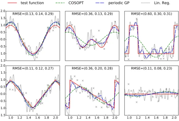
Figure 1 Plots of the benchmark test functions, observation points and fitted models.For an improved visibility, the plotting region is limited to one period. The RMSE is computed using a grid of 500 evenly spaced points spanning[0,3], and the values indicated on each subplot correspond respectively to COSOPT, the periodic Gaussian process model and linear regression. The Python code used to generate this figure is provided as Jupyter notebook inSupplemental Information 3.
The last part of this introduction is dedicated to a motivating example. In ‘Kernels of Periodic and Aperiodic Subspaces,’ we focus on the construction of periodic and aperiodic kernels and on the associated model decomposition. ‘Application to Matérn Kernels’ details how to perform the required computations for kernels from the Matérn familly. ‘Quantifying the Periodicity t’ introduces a new criterion for measuring the periodicity of the signal. Finally, the last section illustrates the proposed approach on a biological case study where we detect, amongst the entire genome, the genes showing a cyclic expression.
The examples and the results presented in this article have been generated with the version 0.8 of the python Gaussian process toolbox GPy. This toolbox, in which we have implemented the periodic kernels discussed here, can be downloaded at
http://github.com/SheffieldML/GPy. Furthermore, the code generating theFigs. 1–3is provided in theSupplemental Information 3as Jupyter notebooks.
Motivating example
To illustrate the challenges of determining a periodic function, we first consider a benchmark of six one dimensional periodic test functions (see Fig. 1andAppendix A). These functions include a broad variety of shapes so that we can understand the effect of shape on methods with different modelling assumptions. A setX=(x1,...,x50) of equally
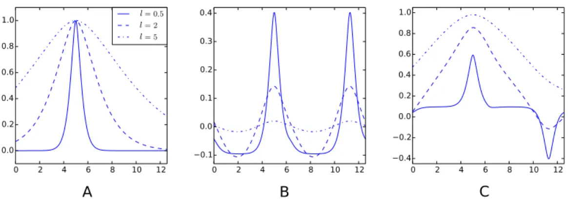
Figure 2 Examples of decompositions of a kernel as a sum of a periodic and aperiodic sub-kernels.
(A) Matérn 3/2 kernelk(.,5). (B) Periodic sub-kernelkp(.,5). (C) Aperiodic sub-kernelka(.,5). For these
plots, one of the kernels variables is fixed to 5. The three graphs on each plot correspond to a different value of the lengthscale parameterℓ. The input space isD= [0,4π]and the cut-off frequency isq=20. The Python code used to generate this figure is provided as Jupyter notebook inSupplemental Informa-tion 3.
Figure 3 Decomposition of a Gaussian process fit. (A) full modelm; (B) periodic portionmpand (C)
aperiodic portionma. Our decomposition allows for recognition of both periodic and aperiodic parts. In
this case maximum likelihood estimation was used to determine the parameters of the kernel, we recov-ered (σp2,ℓp,σa2,ℓa)=(52.96,5.99,1.18,47.79). The Python code used to generate this figure is provided as
Jupyter notebook inSupplemental Information 3.
notations). We consider three different modelling approaches to compare the facets of different approaches based on harmonic analysis:
• COSOPT (Straume, 2004), which fits cosine basis functions to the data, • Linear regression in the weights of a truncated Fourier expansion, • Gaussian process regression with a periodic kernel.
COSOPT. COSOPT is a method that is commonly used in biostatistics for detecting periodically expressed genes (Hughes et al., 2009;Amaral & Johnston, 2012). It assumes the following model for the signal:
y(x)=α+βcos(ωx+ϕ)+ε, (2)
Linear regression.We fit a more general model with a basis of sines and cosines with periods 1,1/2...,1/20 to account for periodic signal that does not correspond to a pure sinusoidal signal.
y(x)=α+
20
X
i=1
βicos(2πix)+
20
X
i=1
γisin(2πix)+ε. (3)
Again, model parameters are fitted by minimizing the mean square error which corresponds to linear regression over the basis weights.
Gaussian Process with periodic covariance function.We fit a Gaussian process model with an underlying periodic kernel. We consider a model,
y(x)=α+yp(x)+ε, (4)
whereypis a Gaussian process and whereαshould be interpreted as a Gaussian random
variable with zero mean and varianceσα2. The periodicity of the phenomenon is taken into account by choosing a processypsuch that the samples are periodic functions. This can be
achieved with a kernel such as
kp(x,x′)=σ2exp −
sin2 ω(x−x′) ℓ
!
(5)
or with the kernels discussed later in the article. For this example we choose the periodic Matérn 3/2 kernel which is represented in Fig. 2B. For any kernel choice, the Gaussian process regression model can be summarized by the mean and variance of the conditional distribution:
m(x)=E[y(x)|y(X) =F] =k(x,X)(k(X,X)+τ2I)−1F
v(x)=Var[y(x)|y(X) =F] =k(x,x)−k(x,X)(k(X,X)+τ2I)−1k(X,x) (6)
wherek=σα2+kpandI is the 50×50 identity matrix. In this expression, we introduced
matrix notation fork: ifAandBare vectors of lengthnandm, thenk(A,B) is an×m
matrix with entriesk(A,B)i,j=k(Ai,Bj). The parameters of the model (σα2,σ2,ℓ,τ2) can
be obtained by maximum likelihood estimation.
The models fitted with COSOPT, linear regression and the periodic Gaussian process model are compared inFig. 1. It can be seen that the latter clearly outperforms the other models since it can approximate non sinusoidal patterns (in opposition to COSOPT) while offering a good noise filtering (no high frequencies oscillations corresponding to noise overfitting such as for linear regression).
The Gaussian process model gives an effective non-parametric fit to the different functions. In terms of root mean square error (RMSE) in each case, it is either the best performing method, or it performs nearly as well as the best performing method. Both linear regression and COSOPT can fail catastrophically on one or more of these examples.
to consider a pseudo-periodic Gaussian process y =y1+yp with a kernel given by
the sum of a usual kernel k1 and a periodic one kp (see e.g., Rasmussen & Williams,
(2006)). Such a construction allows decomposition of the model into a sum of sub-models m(x)=E[y1(x)|y(X) =F] +E[yp(x)|y(X) =F]where the latter is periodic (see
‘Decomposition in periodic and aperiodic sub-models’ for more details). However, the periodic part of the signal is scattered over the two sub-models so it is not fully represented by the periodic sub-model. It would therefore be desirable to introduce new covariance structures that allow an appropriate decomposition in periodic and non-periodic sub-models in order to tackle periodicity estimation for pseudo-periodic signals.
KERNELS OF PERIODIC AND APERIODIC SUBSPACES
The challenge of creating a pair of kernels that stand respectively for the periodic and aperiodic components of the signal can be tackled using the RKHS framework. We detail in this section how decomposing a RKHS into a subspace of periodic functions and its orthogonal complement leads to periodic and aperiodic sub-kernels.Fourier basis in RKHS
We assume in this section that the spaceHpspanned by a truncated Fourier basis
B(x)=
sin 2
π λ x
,...,cos 2
π λ qx
⊤
(7)
is a subspace of the RKHSH. Under this hypothesis, it is straightforward to confirm that the reproducing kernel ofHpis
kp(x,x′)=B⊤(x)G−1B(x′) (8)
whereGis the Gram matrix ofBinH:Gi,j=
Bi,Bj
H. Hereafter, we will refer tokpas the
periodic kernel. In practice, the computation ofkprequires computation of the inner product
between sine and cosine functions inH. We will see in the next section that these computa-tions can be done analytically for Matérn kernels. For other kernels, a more comprehensive list of RKHS inner products can be found inBerlinet & Thomas-Agnan(2004, Chap. 7).
The orthogonal complement ofHpinHcan be interpreted as a subspaceHaofaperiodic
functions. By construction, its kernel iska=k−kp(Berlinet & Thomas-Agnan, 2004). An
illustration of the decomposition of Matérn 3/2 kernels is given inFig. 2. The decomposition of the kernel comes with a decomposition of the associated Gaussian process in to two independent processes and the overall decompositions can be summarised as follow:
H=Hp+⊥Ha↔k=kp+ka↔y=yp+yya. (9)
Many stationary covariance functions depend on two parameters: a variance parameter σ2, which represents the vertical scale of the process and a lengthscale parameter,ℓ, which represents the horizontal scale of the process. The sub-kernels ka andkp inherit these
parameters (through the Gram matrixG for the latter). However, the decomposition
in order to increase the flexibility of the model. The new set of parameters of k is then (σp2,ℓp,σa2,ℓa) with an extra parameterλif the period is not known.
Such reparametrisations of kp andka induce changes in the norms ofHp andHa.
However, if the values of the parameters are not equal to zero or+∞, these spaces still consist of the same elements soHp∩Ha=∅. This implies that the RKHS generated by
kp+kacorresponds toHp+Hawhere the latter are still orthogonal but endowed with a
different norm. Nevertheless, the approach is philosophically different since we buildHby adding two spaces orthogonally whereas inEq. (9)we decompose an existing spaceHinto orthogonal subspaces.
Decomposition in periodic and aperiodic sub-models
The expressiony=yp+yaofEq. (9)allows to introduce two sub-models corresponding
to conditional distributions: a periodic one yp(x)|y(X) = F and an aperiodic one
ya(x)|y(X) = F. These two distributions are Gaussian and their mean and variance
are given by the usual Gaussian process conditioning formulas
mp(x)=E[yp(x)|y(X) =F] =kp(x,X)k(X,X)−1F
ma(x)=E[ya(x)|y(X) =F] =ka(x,X)k(X,X)−1F,
(10)
vp(x)=Var[yp(x)|y(X) =F] =kp(x,x)−kp(x,X)k(X,X)−1kp(X,x)
va(x)=Var[ya(x)|y(X) =F] =ka(x,x)−ka(x,X)k(X,X)−1ka(X,x).
(11)
The linearity of the expectation ensures that the sum of the sub-models means is equal to the full model mean:
m(x)=E[yp(x)+ya(x)|y(X) =F] =E[yp(x)|y(X) =F] +E[ya(x)|y(X) =F]
=mp(x)+ma(x) (12)
so mp andma can be interpreted as the decomposition of minto it’s periodic and
aperiodic components. However, there is no similar decomposition of the variance:
v(x)6=vp(x)+va(x) sinceypandyaare not independent given the observations.
The sub-models can be interpreted as usual Gaussian process models with correlated noise. For example,mpis the best predictor based on kernelkpwith an observational noise
given byka. For a detailed discussion on the decomposition of models based on a sum of
kernels, seeDurrande, Ginsbourger & Roustant (2012).
We now illustrate this model decomposition on the test functionf(x)=sin(x)+x/20 defined over[0,20].Figure 3shows the obtained model after estimating (σp2,ℓp,σa2,ℓa) of a decomposed Matérn 5/2 kernel. In this example, the estimated values of the lengthscales are very different allowing the model to capture efficiently the periodic component of the signal and the low frequency trend.
APPLICATION TO MATÉRN KERNELS
as the non-differentiable Ornstein–Uhlenbeck covariance. In this section, we show how the Matérn class of covariance functions can be decomposed into periodic and aperiodic subspaces in the RKHS.
Matérn kernels k are stationary kernels, which means that they only depend on the distance between the points at which they are evaluated: k(x,y)=˜k(|x−y|). They are often introduced by the spectral density of˜k (Stein, 1999):
S(ω)= Ŵ(ν)ℓ
2ν
2σ2√π Ŵ(ν+1/2)(2ν)ν
2 ν ℓ2 +ω
2ν+1/2
!−1
. (13)
Three parameters can be found in this equation:νwhich tunes the differentiability of˜k,ℓ which corresponds to a lengthscale parameter andσ2that is homogeneous to a variance.
The actual expressions of Matérn kernels are simple when the parameterνis half-integer. Forν=1/2,3/2,5/2 we have
k1/2(x,x′)=σ2exp
−|x−x ′|
ℓ
k3/2(x,x′)=σ2 1+
√
3|x−x′| ℓ
! exp −
√
3|x−x′| ℓ
!
k5/2(x,x′)=σ2 1+
√
5|x−x′|
ℓ +
5|x−x′|2
3ℓ2 !
exp − √
5|x−x′| ℓ
!
.
(14)
Here the parametersℓandσ2respectively correspond to a rescaling of the abscissa and or-dinate axis. Forν=1/2 one can recognise the expression of the exponential kernel (i.e., the covariance of the Ornstein–Uhlenbeck process) and the limit case ν→ ∞corresponds to the squared exponential covariance function (Rasmussen & Williams, 2006).
As stated in Porcu & Stein (2012 Theorem 9.1) and Wendland (2005), the RKHS generated by kν coincides with the Sobolev spaceW2ν+1/2. Since the elements of the
Fourier basis areC∞, they belong to the Sobolev space and thus to Matérn RKHS. The hypothesisHp⊂Hmade in ‘Kernels of Periodic and Aperiodic Subspaces’ is thus fulfilled and all previous results apply.
Furthermore, the connection between Matérn kernels and autoregressive processes allows us to derive the expression of the RKHS inner product. As detailed inAppendix B, we obtain for an input spaceD= [a,b]:
Matérn 1/2 (exponential kernel)
g,h H1/2=
ℓ 2σ2
Z b
a
1
ℓg+g
′ 1
ℓh+h ′
dt+ 1
σ2g(a)h(a). (15)
Matérn 3/2
g,hH3/2 = ℓ
3
12√3σ2 Z b
a
3 ℓ2g+2
√ 3 ℓ g
′+g′′ !
3 ℓ2h+2
√ 3 ℓ h
′+h′′ !
dt
+ 1
σ2g(a)h(a)+ ℓ2 3σ2g
Matérn 5/2
g,h H5/2 =
Z b
a
Lt(g)Lt(h)dt+
9
8σ2g(a)h(a)+ 9ℓ4 200σ2g(a)
′′h′′(a)
+ 3ℓ
2
5σ2
g′(a)h′(a)+1 8g
′′(a)h(a)+1 8g(a)h
′′(a)
(17)
where
Lt(g)=
s 3ℓ5 400√5σ2
5√5 ℓ3 g(t)+
15 ℓ2g
′(t)+3 √
5 ℓ g
′′(t)+g′′′(t) !
.
Although these expressions are direct consequences ofDoob (1953)andHájek (1962), they cannot be found in the literature to the best of our knowledge.
The knowledge of these inner products allow us to compute the Gram matrixGand thus the sub-kernelskpandka. A result of great practical interest is that inner products between
the basis functions have a closed form expression. Indeed, all the elements of the basis can be written in the form cos(ωx+ϕ) and, using the notationLx for the linear operators in
the inner product integrals (seeEq. (17)), we obtain:
Lx(cos(ωx+ϕ))=
X
i
αicos(ωx+ϕ)(i)=
X
i
αiωicos
ωx+ϕ+iπ 2
. (18)
The latter can be factorised in a single cosineρcos(ωx+φ) with
ρ= q
r2
c +rs2, φ=
(
arcsin(rs/ρ) if rc≥0
arcsin(rs/ρ)+π if rc<0
(19)
where
rc=
X
i
αiωicos
ϕ+iπ
2
and rs=
X
i
αiωisin
ϕ+iπ
2
.
Eventually, the computation of the inner product between functions of the basis boils down to the integration of a product of two cosines, which can be solved by linearisation.
QUANTIFYING THE PERIODICITY
The decomposition of the model into a sum of sub-models is useful for quantifying the periodicity of the pseudo-periodic signals. In this section, we propose a criterion based on the ratio of signal variance explained by the sub-models.
In sensitivity analysis, a common approach for measuring the effect of a set of variables
x1,...,xnon the output of a multivariate functionf(x1,...,xn) is to introduce a random
vectorR=(r1,...,rn) with values in the input space off and to define the variance explained
by a subset of variablesxI=(xI1,...,xIm) asVI=Var E f(R)|RI
We now apply these two principles to define a periodicity ratio based on the sub-models. LetRbe a random variable defined over the input space andyp,yabe the periodic and
aperiodic components of the conditional process y given the data-points.ypandyaare
normally distributed with respective mean and variance (mp, vp), (ma, va) and their
covariance is given by Cov(yp(x),ya(x′))= −kp(x,X)k(X,X)−1ka(x′). To quantify the
periodicity of the signal we introduce the following periodicity ratio:
S= VarR[yp(R)]
VarR[yp(R)+ya(R)]
. (20)
Note thatScannot be interpreted as a the percentage of periodicity of the signal in a rigorous way since VarR[yp(R)+ya(R)] 6=VarR[yp(R)] +VarR[ya(R)]. As a consequence,
this ratio can be greater than 1.
For the model shown inFig. 3, the mean and standard deviation ofSare respectively 0.86 and 0.01.
APPLICATION TO GENE EXPRESSION ANALYSIS
The 24 h cycle of days can be observed in the oscillations of biological mechanisms at many spatial scales. This phenomenon, called the circadian rhythm, can for example be seen at a microscopic level on gene expression changes within cells and tissues. The cellular mechanism ensuring this periodic behaviour is called the circadian clock. For arabidopsis, which is a widely used organism in plant biology and genetics, the study of the circadian clock at a gene level shows an auto-regulatory system involving several genes (Ding et al., 2007). As argued byEdwards et al. (2006), it is believed that the genes involved in the oscillatory mechanism have a cyclic expression so the detection of periodically expressed genes is of great interest for completing current models.
Within each cell, protein-coding genes are transcribed into messenger RNA molecules which are used for protein synthesis. To quantify the expression of a specific protein-coding gene it is possible to measure the concentration of messenger RNA molecules associated with this gene. Microarray analysis and RNA-sequencing are two examples of methods that take advantage of this principle.
The dataset (see http://millar.bio.ed.ac.uk/data.htm) considered here was originally studied by Edwards et al. (2006). It corresponds to gene expression for nine day old arabidopsis seedlings. After eight days under a 12 h-light/12 h-dark cycle, the seedlings are transferred into constant light. A microarray analysis is performed every four hours, from 26 to 74 h after the last dark-light transition, to monitor the expression of 22,810 genes.Edwards et al. (2006)use COSOPT (Straume, 2004) for detecting periodic genes and identify a subset of 3,504 periodically expressed genes, with an estimated period between 20 and 28 h.
We now apply to this dataset the method described in the previous sections. The kernel we consider is a sum of a periodic and aperiodic Matérn 3/2 kernel plus a delta function to reflect observation noise:
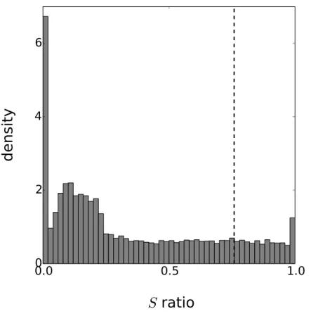
Figure 4 Distribution of the periodicity ratio over all genes according to the Gaussian process mod-els.The cut-off ratio determining if genes are labelled as periodic or not is represented by a vertical dashed line.
Although the cycle of the circadian clock is known to be around 24 h, circadian rhythms often depart from this figure (indeedcirca diais Latin foraround a day) so we estimated the parameterλto determine the actual period. The final parametrisation ofk is based on six variables: (σp2,ℓp,σa2,ℓa,τ2,λ). For each gene, the values of these parameters are estimated
using maximum likelihood. The optimization is based on the standard options of the GPy toolkit with the following boundary limits for the parameters:σp, σa≥0;ℓp, ℓa∈ [10,60]; τ2∈ [10−5,0.75]andλ∈ [20,28]. Furthermore, 50 random restarts are performed for each
optimization to limit the effects of local minima.
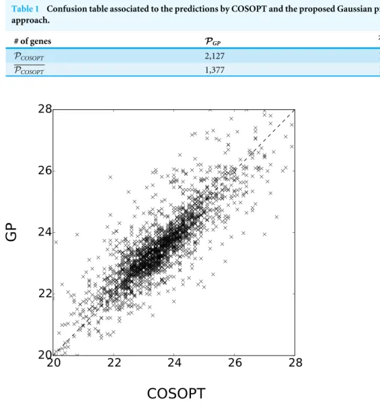
Table 1 Confusion table associated to the predictions by COSOPT and the proposed Gaussian process approach.
# of genes PGP PGP
PCOSOPT 2,127 1,377
PCOSOPT 1,377 17,929
Figure 5 Comparison of Estimated periods for the genes inPGP∩PCOSOPT. The coefficient of
determi-nation ofx→x(dashed line) is 0.69.
LetPCOSOPTandPGPbe the sets of selected periodic genes respectively byEdwards et al. (2006)and the method presented here and letPCOSOPTandPGPdenote their complements. The overlap between these sets is summarised inTable 1. Although the results cannot be compared to any ground truth, the methods seem coherent since 88% of the genes share the same label. Furthermore, the estimated value of the periodλis consistent for the genes labelled as periodic by the two methods, as seen inFig. 5.
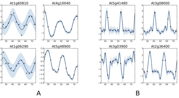
Figure 6 Examples of genes with different labels.(A) corresponds to genes labelled as periodic by COSOPT but not by the Gaussian process approach, whereas in (B) they are labelled as periodic only by the latter. In (A, B), the four selected genes are those with the highest periodic part according to the method that labels them as periodic. The titles of the graphs correspond to the name of the genes (AGI convention).
corresponding either to noise or trend. For these genes, the value of the periodicity ratio is: 0.74 (0.10), 0.74 (0.15), 0.63 (0.11), 0.67 (0.05) (means and standard deviations, clockwise from top left) which is close to the classification boundary. On the other hand, the genes selected only by the Gaussian process approach show a strong periodic signal (we have for all genesS=1.01 (0.01)) with sharp spikes. We note fromFig. 6Bthat there is always at least one observation associated with each spike, which ensures that the behaviour of the Gaussian process models cannot simply be interpreted as overfitting. The reason COSOPT is not able to identify these signals as periodic is that it is based on a single cosine function which makes it inadequate for fitting non sinusoidal periodic functions. This is typically the case for gene expressions with spikes as inFig. 6B, but it can also be seen on the test functions ofFig. 1.
This comparison shows very promising results, both for the capability of the proposed method to handle large datasets and for the quality of the results. Furthermore, we believe that the spike shape of the newly discovered genes may be of particular interest for understanding the mechanism of the circadian clock. The full results, as well as the original dataset, can be found in theSupplemental Information.
CONCLUSION
The main purpose of this article is to introduce a new approach for estimating, extracting and quantifying the periodic component of a pseudo-periodic functionf given some noisy observationsyi=f(xi)+ε. The proposed method is typical in that it corresponds to the
be dealt with elegantly. Previous theoretical results from the mid-1900s allowed us to derive the expressions of the inner product of RKHS based on Matérn kernels. Given these results, it was then possible to define a periodic kernelkpand to decomposek as a sum of
sub-kernelsk=kp+ka.
We illustrated three fundamental features of the proposed kernels for Gaussian process modelling. First, as we have seen on the benchmark examples, they allowed us to approximate periodic non-sinusoidal patterns while retaining appropriate filtering of the noise. Second, they provided a natural decomposition of the Gaussian process model as a sum of periodic and aperiodic sub-models. Third, they can be reparametrised to define a wider family of kernel which is of particular interest for decoupling the assumptions on the behaviour of the periodic and aperiodic part of the signal.
The probabilistic interpretation of the decomposition in sub-models is of great importance when it comes to define a criterion that quantifies the periodicity off while taking into account the uncertainty about it. This goal was achieved by applying methods commonly used in Gaussian process based sensitivity analysis to define a periodicity ratio.
Although the proposed method can be applied to any time series data, this work has originally been motivated by the detection of periodically expressed genes. In practice, listing such genes is a key step for a better understanding of the circadian clock mechanism at the gene level. The effectiveness of the method is illustrated on such data in the last section. The results we obtained are consistent with the literature but they also feature some new genes with a strong periodic component. This suggests that the approach described here is not only theoretically elegant but also efficient in practice.
As a final remark, we would like to stress that the proposed method is fully compatible with all the features of Gaussian processes, from the combination of one-dimensional periodic kernels to obtain periodic kernels in higher dimension to the use of sparse methods when the number of observation becomes large. By implementing our new method within the GPy package for Gaussian process inference we have access to these generalisations along with effective methods for parameter estimation. An interesting future direction would be to incorporate the proposed kernel into the ‘Automated Statistician’ project (Lloyd et al., 2014;Duvenaud et al., 2013), which searches over grammars of kernels.
APPENDIX A. DETAILS ON TEST FUNCTIONS
The test functions shown inFig. 1are 1-periodic. Their expressions forx∈ [0,1) are (from top left, in a clockwise order):
f1(x)=cos(2πx)
f2(x)=1/2cos(2πx)+1/2cos(4πx)
f3(x)=
(
1 if x∈ [0,0.2] −1 if x∈(0.2,1)
f4(x)=4|x−0.5| +1 f5(x)=1−2x f6(x)=0.
APPENDIX B. NORMS IN MATÉRN RKHS
Autoregressive processes and RKHS norms
A process is said to be autoregressive (AR) if the spectral density of the kernel
S(ω)= 1 2π
Z
R
k(t)e−iωtdt (23)
can be written as a function of the form
S(ω)= 1
Pm
k=0αk(iω)k
2 (24)
where the polynomialPm
k=0αkxk is real with no zeros in the right half of the complex
planDoob (1953). Hereafter we assume thatm≥1 and thatα0,αm6=0.
For such kernels, the inner product of the associated RKHSHis given byHájek (1962), Kailath (1971)andParzen (1961)
h,gH= Z b
a
(Lth)(Ltg)dt+2
X
0≤j,k≤m−1
j+k even
dj,kh(j)(a)g(k)(a) (25)
where
Lth= m
X
k=0
αkh(k)(t) and dj,k=
min(j,k)
X
i=max(0,j+k+1−n)
(−1)(j−i)α
iαj+k+1−i.
We show in the next section that the Matérn kernels correspond to autoregressive kernels and, for the usual values ofν, we derive the norm of the associated RKHS.
Application to Matérn kernels
Following the pattern exposed inDoob(1953, p. 542), the spectral density of a Matérn kernel (Eq. (13)) can be written as the density of an AR process whenν+1/2 is an integer. Indeed, the roots of the polynomial 2ν
ℓ2 +ω2are conjugate pairs so it can be expressed as the squared module of a complex number
2ν ℓ2+ω
2
= ω+i √
2ν ℓ
!
ω−i √ 2ν ℓ ! =
ω+i √ 2ν ℓ 2 . (26)
Multiplying by iand taking the conjugate of the quantity inside the module, we finally obtain a polynomial iniωwith all roots in the left half of the complex plan:
2ν ℓ2+ω
2 =
iω+ √ 2ν ℓ 2 ⇒ 2 ν ℓ2+ω
2(ν+1/2)
= √ 2ν ℓ +iω
!(ν+1/2) 2 . (27)
Plugging this expression intoEq. (13), we obtain the desired expression ofSν:
Sν(ω)=
1 q
Ŵ(ν)ℓ2ν
2σ2√π Ŵ(ν+1/2)(2ν)ν √
2ν
ℓ +iω
(ν+1/2)
UsingŴ(ν)=22ν(2−ν1−(ν1)−!√1/π2)!, one can derive the following expression of the coefficientsαk:
αk=
s
(2ν−1)!νν
σ2(ν−1/2)!22νC k ν+1/2
ℓ √
2ν k−1/2
. (29)
Theses values ofαk can be plugged intoEq. (25)to obtain the expression of the RKHS
inner product. The results forν∈ {1/2,3/2,5/2}is given by Eqs. (15)–(17)in the main body of the article.
ADDITIONAL INFORMATION AND DECLARATIONS
Funding
Support was provided by the BioPreDynProject (Knowledge Based Bio-Economy EU grant Ref 289434) and the BBSRC grant BB/1004769/1. James Hensman was funded by an MRC career development fellowship. The funders had no role in study design, data collection and analysis, decision to publish, or preparation of the manuscript.
Grant Disclosures
The following grant information was disclosed by the authors: BioPreDynProject: Ref 289434.
BBSRC: BB/1004769/1.
Competing Interests
The authors declare there are no competing interests.
Author Contributions
• Nicolas Durrande and James Hensman conceived and designed the experiments, performed the experiments, analyzed the data, contributed reagents/materials/analysis tools, wrote the paper, prepared figures and/or tables, performed the computation work, reviewed drafts of the paper.
• Magnus Rattray and Neil D. Lawrence conceived and designed the experiments, analyzed the data, contributed reagents/materials/analysis tools, wrote the paper, performed the computation work, reviewed drafts of the paper.
Data Availability
The following information was supplied regarding data availability: GitHub:https://github.com/SheffieldML.
Supplemental Information
Supplemental information for this article can be found online athttp://dx.doi.org/10.7717/ peerj-cs.50#supplemental-information.
REFERENCES
Amaral I, Johnston I. 2012.Circadian expression of clock and putative
clock-controlled genes in skeletal muscle of the zebrafish.American Journal of Physiology
Aronszajn N. 1950.Theory of reproducing kernels.Transactions of the American Mathematical Society68(3):337–404DOI 10.1090/S0002-9947-1950-0051437-7. Berlinet A, Thomas-Agnan C. 2004.Reproducing kernel Hilbert spaces in probability and
statistics. Dordrecht: Kluwer Academic Publishers.
Ding Z, Doyle MR, Amasino RM, Davis SJ. 2007.A complex genetic interaction between Arabidopsis thaliana TOC1 and CCA1/LHY in driving the circadian clock and in output regulation.Genetics176(3):1501–1510DOI 10.1534/genetics.107.072769. Doob JL. 1953.Stochastic processes. Vol. 101. New York: John Wiley & Sons.
Durrande N, Ginsbourger D, Roustant O. 2012.Additive covariance kernels for high-dimensional Gaussian process modeling.Annales de la faculté des Sciences de Toulouse
XXI:481–499.
Duvenaud D, Lloyd J, Grosse R, Tenenbaum J, Zoubin G. 2013.Structure discovery in nonparametric regression through compositional kernel search. In:Proceedings of the 30th international conference on machine learning, 1166–1174.
Edwards KD, Anderson PE, Hall A, Salathia NS, Locke JCW, Lynn JR, Straume M, Smith JQ, Millar AJ. 2006.FLOWERING LOCUS C mediates natural variation in the high-temperature response of the Arabidopsis circadian clock.The Plant Cell Online18(3):639–650DOI 10.1105/tpc.105.038315.
Hájek J. 1962.On linear statistical problems in stochastic processes.Czechoslovak Mathematical Journal12(87):404–444.
Hartley HO. 1949.Tests of significance in harmonic analysis.Biometrika36(1):194–201
DOI 10.1093/biomet/36.1-2.194.
Hughes M, DiTacchio L, Hayes K, Vollmers C, Pulivarthy S, Baggs J, Panda S, Ho-genesch J. 2009.Harmonics of circadian gene transcription in mammals.PLoS Genetics5(4):e1000442DOI 10.1371/journal.pgen.1000442.
Kailath T. 1971.RKHS approach to detection and estimation problems–I: deterministic signals in Gaussian noise.IEEE Transactions on Information Theory17(5):530–549
DOI 10.1109/TIT.1971.1054673.
Leahy DA, Darbro W, Elsner RF, Weisskopf MC, Kahn S, Sutherland PG, Grindlay JE. 1983.On searches for pulsed emission with application to four globular cluster X-ray sources-NGC 1851, 6441, 6624, and 6712.Astrophysical Journal266:160–170
DOI 10.1086/160766.
Lloyd JR, Duvenaud D, Grosse R, Tenenbaum J, Ghahramani Z. 2014.Automatic construction and natural-language description of nonparametric regression models. In:Twenty-eighth AAAI conference on artificial intelligence. Palo Alto: Association for the Advancement of Artificial Intelligence.
Marrel A, Iooss B, Laurent B, Roustant O. 2009.Calculations of sobol indices for the gaussian process metamodel.Reliability Engineering & System Safety94(3):742–751
DOI 10.1016/j.ress.2008.07.008.
Matheron G. 1963.Principles of geostatistics.Economic Geology58(8):1246–1266
Oakley JE, O’Hagan A. 2004.Probabilistic sensitivity analysis of complex models: a Bayesian approach.Journal of the Royal Statistical Society: Series B (Statistical Methodology)66(3):751–769 DOI 10.1111/j.1467-9868.2004.05304.x.
Parzen E. 1961.An approach to time series analysis.The Annals of Mathematical Statistics
32(4):951–989.
Porcu E, Stein ML. 2012.On some local, global and regularity behaviour of some classes of covariance functions. Berlin Heidelberg: Springer, 221–238.
Rasmussen CE, Williams C. 2006.Gaussian processes for machine learning. Cambridge: MIT Press.
Scheuerer M, Schaback R, Schlather M. 2011.Interpolation of spatial data—a stochastic or a deterministic problem?Technical report. Universität Göttingen.
Schuster A. 1898.On the investigation of hidden periodicities with application to a supposed 26 day period of meteorological phenomena.Terrestrial Magnetism
3(1):13–41DOI 10.1029/TM003i001p00013.
Stein ML. 1999.Interpolation of Spatial Data: some theory for kriging. Berlin Heidelberg: Springer Verlag.
Stellingwerf RF. 1978.Period determination using phase dispersion minimization.
Astrophysical Journal 224:953–960DOI 10.1086/156444.
Straume M. 2004.DNA microarray time series analysis: automated statistical assess-ment of circadian rhythms in gene expression patterning.Methods in Enzymology
383:149–166DOI 10.1016/S0076-6879(04)83007-6.
Thomson W. 1878.Harmonic analyzer.Proceedings of the Royal Society of London
27(185–189):371–373DOI 10.1098/rspl.1878.0062.
Troutman BM. 1979.Some results in periodic autoregression.Biometrika66(2):219–228
DOI 10.1093/biomet/66.2.219.
Vecchia AV. 1985.Maximum likelihood estimation for periodic autoregressive moving average models.Technometrics27(4):375–384DOI 10.1080/00401706.1985.10488076. Wahba G. 1990.Spline models for observational data. Vol. 59. Philadelphia: Society for
Industrial Mathematics.