Markcilei Lima Dan
[email protected] Federal Institute of Espírito Santo Mechanical Department Cachoeiro de Itapemirim 29300-970 Espírito Santo, BrazilCarlos Friedrich Loeffler Neto
[email protected] Federal University of Espírito Santo Mechanical Engineering Department Vitória 29075-910 Espírito Santo, BrazilWebe João Mansur
[email protected] Federal University of Rio de Janeiro Civil Engineering Department Rio de Janeiro 21945-970 Rio de Janeiro, BrazilA Transformation of Variables
Technique Applicable to the
Boundary Element Method to
Simulate a Special Class of
Diffusive-Advective Potential Problems
This paper describes a novel Boundary Element Technique developed for application to one-dimensional and a class of two-dimensional diffusive-advective potential problems. It is based on transformation of variable procedure to establish an integral equation inverse sentence, dealing only with boundary variables, using a fundamental solution associated with a diffusive problem. To apply the technique described here, the original differential equation is rewritten and flow potential functions are employed to contract terms which appear in the original equation, giving as a result an equivalent equation expressed in terms of the derivative of the product of two functions. This new form of the governing equation, together with the proposed transformation of variables is quite convenient for the application of the boundary element methodology: a very simple discretization procedure arises; the resulting algorithms require low CPU time and the numerical results are quite accurate.
Keywords: Boundary Element Method, potential problems, diffusive-advective equation, fluid flow modeling
Introduction1
Despite the great amount of research work developed in the last thirty years, there is still a wide unexplored field of research concerning applications of Boundary Element Method (BEM) to Engineering. There are important classes of problems which require more consistent approaches; in particular, one can mention the area of study of Transport Phenomena (White, 1986) and specifically diffusive-advective problems (Ramachandran, 1994). The most consistent and elegant formulation to deal with diffusive-advective problems in two-dimensions employs a fundamental solution of a similar diffusive-advective problem, with a concentrated source applied at a domain point (Honna et al., 1985, and also Wrobel and De Figueiredo, 1991). Such formulation is capable of solving with great accuracy problems where the velocity field is constant; however, the approach is not adequate anymore if the velocity field is dependent on spatial coordinates. Another drawback concerning this formulation is the difficulty to apply it to time dependent problems, as the fundamental solution for this case is quite cumbersome.
The first BEM general formulation developed to diffusive-advective problems was presented by Partridge et al. in 1992. This formulation is based on the Dual Reciprocity procedure proposed originally by Nardine and Brebbia (1982). Utilizing a diffusive fundamental solution, the formulation presented by Partridge et al, overcame the restriction of the previous formulation which could only be applied if the velocity field was constant; however, it presented a serious limitation when accuracy is concerned, its application being recommended only for fluid flow with low Peclet numbers (Bejan, 1993; Bennet and Myers, 1983).
Following the Dual Reciprocity Formulation (DRF) guidelines, Loeffler and Mansur (2003) proposed a novel procedure called Quasi-Dual Reciprocity formulation (QDR). The structure of the QDR is similar to that of the Dual-Reciprocity, especially when the
Paper received 13 May 2011. Paper accepted 23 November 2011. Technical Editor: Horácio Vielmo
use of auxiliary interpolation radial basis functions is concerned (Karur and Ramachandran, 1994; Partridge, 1997); however, a special treatment concerning the advective terms was proposed aiming at improving the accuracy of the numerical results for high Peclet numbers.
In the present work, a novel approach is proposed, named Harmonic Transformation Technique (HTT). This new approach also employs a diffusive fundamental solution like the DRF and the QDR, but it employs operational procedures which include a special transformation of variables that makes the computational process quicker and accurate. This transformation is based on the governing equation equivalence between potential advective problems and inhomogeneous scalar problems, that is, Laplace´s problems; this equation can be easily written in the inverse integral form if strategic operations put it in harmonic form.
Nomenclature
B = constant defined by Eq. (30), kg/(m2 s)
Em = mean error, dimensionless
Ep = nodal error, dimensionless
f = natural boundary condition, ºC m/s
G = global matrix of the Boundary Element Method, dimensionless
H = global matrix of the Boundary Element Method, 1/m
K = thermal diffusivity of the medium, m2/s
L = length of the control volume, m
m = parameter of control of the fluid flow velocity, Eq. (31), 1/s
n = number of boundary elements used in the boundary discretization, dimensionless
Nf = total number of nodal points where the mean error is
calculated, dimensionless
ni = cartesian coordinates of the vector normal to the
boundary, dimensionless
P = global matrix originated from harmonic transformation technique, dimensionless
p = Peclet number, dimensionless
Q = boundary condition prescribed at face 2, in exemple 2, ºc/m
q = derivative of the temperature in the direction normal to the boundary, ºC/m
q = vector containing the nodal value of the derivative of the temperature in the direction normal to the boundary, ºC/m ˆ
q = vector containing the nodal value of the derivative of the transformed variable in the direction normal to the boundary, ºC/m
vi = cartesian component of the velocity field, m/s
vx = cartesian component in the x direction of the velocity
field, m/s
vy = cartesian component in the y direction of the velocity
field, m/s
Greek Symbols
Γ = boundary of the domain where the diffusive-advective potential problem is defined
Γq = region of the boundary where is prescribed the natural
boundary condition
Γu = region of the boundary where is prescribed the essential
boundary condition
η = function of the potential of velocity used to compaction of the governing equation, defined by Eq. (7),
dimensionless
ηηηη = vector containing the nodal value of the function η, dimensionless
θ = temperature, ºC
θ = vector containing nodal value of temperature on
boundary, ºC
θ = temperature prescribed at the boundary (essential boundary condition), ºC
ρ = fluid density, kg/m3
Ψ = transformed variable defined by Eqs. (14) and (15), ºC Ψ = vector containing the nodal value of the transformed
variable in the boundary, ºC
Ψ = homogeneous vector containing a unique nodal value of the transformed variable, ºC
k
Ψ = nodal value of the transformed variable at nodal point k, ºC
Ω = domain where the diffusive-advective potential problem is defined
Basic Problem
The governing equation and boundary conditions can be presented in a more simple form; as mentioned before, the core of HTT is one-dimensional applications. On the other hand, in BEM approaches, it is very common to use two-dimensional codes to solve also more simple situations. For this reason, a mathematical model in two dimensions is presented here.
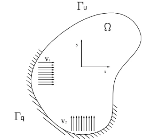
Then, here it is considered a homogeneous fluid medium, with mass movement which permits characterization of a continuous flow, subjected to a temperature gradient. Let Ω be an internal region, delimited by a boundaryΓ, as shown in Fig. 1:
Figure 1. Characterization of the domain Ω and boundaryΓ.
Herein it is assumed incompressible and inviscid flow and steady state conditions (Batchelor, 1967). In this case exists a temperature field θ(x, y) in Ω, governed by a well-known partial differential equation (Incropera and Witt, 1992), presented in Eq. (1) using Einstein’s indicial notation:
ii i i
,
,
K
θ
=
v
θ
(1)In Eq. (1) K is the thermal diffusivity of the medium and v , i
i 1, 2= represents respectively the x and y components of the velocity field.
It is assumed that on Γu and Γq (Γ Γ= ∪u Γq) are known respectively the temperature θ (essential boundary condition) or a function f involving temperature derivative θ, ni i on the direction normal to Γ and the particle velocity component in the normal direction versus θ. The boundary conditions are thus described by:
θ
=
θ
onu
Γ
(essential boundary condition) (2),i i i i
f
=
K
θ
n
+
v n
θ
onΓ
q (natural boundary condition) (3)Governing Equation Compaction
To develop the formulation, it is convenient to rewrite the governing equation, Eq. (1), in a compact form, such that the advective and diffusive parcels can be expressed in terms of the derivative of the product of two functions, as shown by Eq. (4):
q
x y
u
v1
( )
ηθ
, ,
i i=
0
(4)The last expression is the inhomogeneous Laplace´s equation. In this equation
η
(x, y) is a function related to the velocity field existing in the Ω domain. Next it is shown the steps required to reach the contracted form of the governing equation, given by Eq. (4); an expression to computeη
as a function of the velocity field and the thermal diffusivity of the medium is obtained.First, the derivative indicated in Eq. (4) is performed:
ii i i
ηθ
,
+
η
,
θ
,
=
0
(5)Comparing Eq. (5) with Eq. (1), one can see that if
η
obeys the differential equation indicated by Eq. (6), Eq. (5) and Eq. (1) become the same:i i
v
η
,
η
K
= −
(6)The above expression represents a system of two ordinary equations which are used to determine the function
η
, from where one can conclude that Eq. (4) is equivalent to the governing equation, as long as one considersη
given by:(
)
η
=
exp
−
Φ
K
(7)Thus, as Φ,i=vi, the scalar function Φ can be interpreted as a velocity potential.
The transformation presented in Eq. (7) links the general Laplace´s Equation for inhomogeneous medium and the Advective-Diffusive Equation. It is a sufficient condition for one-dimensional cases, but for two-dimensional ones the incompressibility and irrotationality conditions to the fluid flow are required.
The Harmonic Transformation Technique
Starting from the compact form of the governing equation, Eq. (4), it is possible to apply a transformation of variables procedure aiming at simplifying the numerical model formulation. To achieve this goal, one must introduce a new variable Ψ, related to the original variable
θ
according to:i i
Ψ
,
=
ηθ
,
(8)The objective is to write the governing equation in a harmonic equivalent form, suitable to a BEM approach. If Eq. (8) is substituted into Eq. (4), one has:
ii
Ψ
,
=
0
(9)Thus, Ψ is governed by the Laplace equation. The classical BEM procedure (Brebbia, 1978) leads to the following matrix equation:
ˆ
0
H
Ψ
- Gq =
(10)where ˆq=Ψ, ni i. It is necessary now to determine the vectors Ψ and qˆ. The vector qˆ can be determined directly from Eq. (8):
ˆ
q =
η
q
(11)where q in the last equation is the flux of
θ
, i.e.i i
q
=
θ
, n
(12)The function Ψ is also determined from Eq. (8); by application of the chain rule:
i i
Ψ
Ψ
θ
x
θ
x
∂
∂ ∂
∂
=
∂ ∂
(13)Comparing Eq. (13) and Eq. (8), it is easy to understand that the function Ψ must be such that:
Ψ
η
θ
∂
∂
=
(14)Equation (14) cannot be solved analytically, as η(θ) is not known. However, it is possible to establish a scheme to carry out the numerical integration of this equation between two arbitrary points within the Ω domain, as indicated by Eq. (15):
k
k k -1 k -1
Ψ
-
Ψ
=
∫
η
d
θ
(15)If k and k−1 are considered to be two consecutive nodes of a discretized boundary, the following approximation is valid:
k k 1− m
(
k k 1−)
Ψ ≅ Ψ + η θ − θ
(16)In the previous equation
η
m is admitted to be as an intermediate value of the functionη
within the integration interval, for the sake of simplicity. The trapezoidal rule was employed to perform the integration indicated in Eq. (15); the result being that indicated by Eq. (16). Since the equation (16) is the simplest approach to process the integration given by the equation (15), some more accurate schemes could easily be imagined to improve it, especially considering some weighted effect of adjacent nodal values. However, the most effective way to improve the accuracy of this integration without loss of simplicity is the use of boundary elements of the highest order, since the improvement of the proposed scheme would happen naturally.Considering now the boundary being discretized through n constant boundary elements (Brebbia and Walker, 1980) and applying Eq. (16) between the first and last nodes, it is possible to write the following expression:
1 n n1
(
1 n)
Ψ ≅ Ψ + η θ − θ
(17)For the next interval, one can write:
2 1 12
(
2 1)
Ψ ≅ Ψ + η θ − θ
(18)Substituting Eq. (17) into Eq. (18), one has
2 n n1
(
1 n)
12(
2 1)
When this procedure is repeated to all boundary nodes, one obtains the following equations:
1 n n1 1 n
2 n n1 1 n 12 2 1
3 n n1 1 n 12 2 1 23 3 2
4 n n1 1 n 12 2 1 23 3 2 34 4 3
n n n1 1 n 12 2 1 23 3 2 34 4 3 ( n 1) n
(
)
(
)
(
)
(
)
(
)
(
)
(
)
(
)
(
)
(
)
(
)
(
)
(
)
(
) ...
−(
Ψ ≅ Ψ + η θ − θ
Ψ ≅ Ψ + η θ − θ + η θ − θ
Ψ ≅ Ψ + η θ − θ + η θ − θ + η θ − θ
Ψ ≅ Ψ + η θ − θ + η θ − θ + η θ − θ + η θ − θ
Ψ ≅ Ψ + η θ − θ + η θ − θ + η θ − θ + η θ − θ +
+ η
θ
⋮
⋮
⋮
⋮
n
− θ
n 1−)
(20)
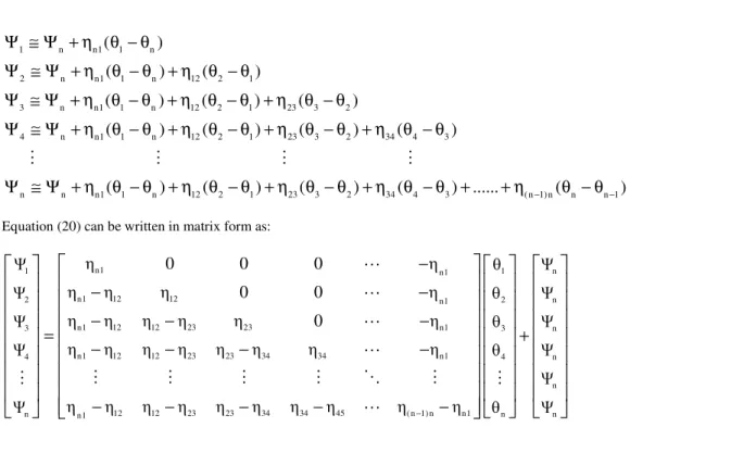
Equation (20) can be written in matrix form as:
n1
1 n1 1
n1 12 12
2 n1 2
n1 12 12 23 23 n1
3 3
n1 12 12 23 23 34 34 n1
4 4
12 12 23 23 34 34 45 ( n 1) n n1
n n1 n
η
0
0
0
η
Ψ
θ
η
η
η
0
0
η
Ψ
θ
η
η
η
η
η
0
η
Ψ
θ
η
η
η
η
η
η
η
η
Ψ
θ
η
η
η
η
η
η
η
η
η
η
Ψ
−θ
−
−
−
−
−
−
=
−
−
−
−
−
−
−
−
−
⋯
⋯
⋯
⋯
⋮
⋮
⋮
⋮
⋱
⋮
⋮
⋮
⋯
n
n
n
n
n
n
Ψ
Ψ
Ψ
Ψ
Ψ
Ψ
+
(21)
Equation (21) is rewritten in compact notation:
Ψ
= P
θ
+
Ψ
(22)Substituting Eq. (22) and Eq. (11) into Eq. (10) it gives:
HP
θ
- G
η
q = -H
Ψ
(23)As
Ψ
is a homogeneous vector, having in mind that the sum of all terms of a row of matrix H is null (Brebbia, 1978) one has:H
Ψ
= 0
(24)Thus, Eq. (23) becomes:
HP
θ
- G
η
q = 0
(25)This last equation can be easily solved by the usual methods employed to solve linear algebraic system of equations. Although the set of equations above refer to a boundary discretized into constant elements, it’s easy to establish new forms to the equations above when higher-order elements are used. In this case, considering the potential function θ written in terms of the local
coordinates (Brebbia, Telles and Wrobel, 1984) and
η
being a known function, the integral in the right-hand-side of Eq. (15) can be performed using standard Gauss quadrature rule. In this way, a new set of equations related to a more precise integration scheme can be obtained.Applications
This topic discussion concerns three test-cases whose analytical solutions are known, thereby used to evaluate the performance of the formulation proposed. In the three applications, it is shown the
behavior of the numerical solution for different mesh refinement and Peclet numbers. Another important point to be highlighted concerning the numerical simulations carried out is related to the need for poles (internal nodes, basis for global interpolation). It is well known in the literature, e.g., Loeffler and Mansur (1987), that the DRF requires the use of poles to improve the representation of domain known or unknown functions; in the present case the advective term. However, the approach proposed here (HTT) does not require poles. The DRF employed sixteen poles homogeneously distributed within the control volume, whereas the HTT and QDR did not use any.
One-Dimensional Fluid Flow with a Constant Velocity Field
The first example consists of a heat transfer problem with a one–dimensional constant velocity field, subjected to the following boundary conditions: null diffusive flux on the horizontal edges, and prescribed temperatures on the vertical ones, as shown in Fig. 2.
Figure 2. Physical and geometrical characteristics of example 1. v
L
x y
fa
c
e
4
fa
c
e
2
face1
v L p
K
= O
The analytical solution of this problem is given by:
px
pL
e
1
e
1
−
θ =
−
(26)px
pL
pe
q
e
1
=
−
(27)In the previous equations, θ is the temperature, q is the
derivative in the direction of the normal to the boundary of a control volume whose boundary coincides with that shown in the Fig. 2 and p is the Peclet number. The results obtained from the numerical simulations are described by graphs which illustrate the behavior of the numerical solution through values of the mean error, described in percentage with respect to the analytical value, the following expression being used in the computations:
p m
f
E E
N
∑
=
(28)where:
at considered po int p
analyt. value numer. value abs
analyt. value
E =
−
(29)In Eq. (28)
N
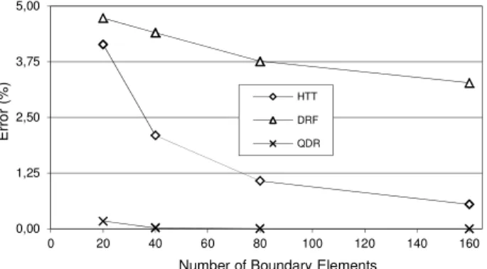
f is the number of nodal points on the face where the temperature or its derivative is computed. Equation (28) will be employed for all examples shown here.Figures 3 and 4 show graphs of numerical results errors versus number of boundary elements, for a fixed Peclet number equal 2. These figures show the good convergence rate of the HTT whose performance is much superior to that of the DRF.
In Fig. 3 it is shown the variation of the percentage error of the numerical results on face 1 versus mesh refinement.
For a coarse mesh, the effect of the approximation shown by Eq. (16) is quite significant, so that the accuracy of the HTT is worse than that of the QDR and DRF. This behavior is credited to the low order interpolation used in Eq. (16). However, as the mesh becomes finer, the accuracy of HTT becomes closer to that of the QDR; in fact, the difference of the two formulations for more than eighty boundary elements is meaningless. Both, HTT and QDR approaches are superior to the DRF, even for this example with low Peclet Number.
Figure 3. Temperature percentage mean error on face 1, versus mesh refinement for Peclet number equal to 2, for example 1.
In what boundary fluxes on the input and output faces are concerned, the results of HTT and QDR approaches become closer than that of temperature results described previously. Although for coarse meshes the HTT have a poor performance, its accuracy improves substantially with mesh refinement; results of HTT and QDR shown in Fig. 4 are coincident for a number of boundary elements higher than eighty. Still better results for HTT may be expected if higher order interpolation is used in Eq. (16), even when a coarse mesh is considered.
Figure 4. Normal flux percentage mean error on face 4 versus mesh refinement for Peclet number equal to 2, for example 1.
Figures 5 and 6 illustrate the performance of the proposed formulation for different Peclet numbers, for a fixed boundary element mesh refinement; one hundred and sixty elements were employed. The solution of diffusive-advective problems is quite sensitive to the variations of the Peclet number. This becomes a serious difficulty to the approaches examined here, which model together the diffusive and the advective phenomena without considering in their mathematical structure the preponderance of one of the processes over the other.
Figure 5 depicts the values of the mean percentage error concerning the computation of the temperatures on face 1. This figure shows that for Peclet Numbers over 4, the DRF presents high errors. It can also be noted that QDR results starts deteriorating for the Peclet Number about 10; as the Peclet number becomes bigger than 10 one can notice a quick increase of the percentage mean error. Errors of the HTT formulation increase slowly with the increase of the Peclet number. Results accuracy is acceptable (error less than 3%) for the range of variation depicted in Fig. 5.
Figure 5. Temperature percentage mean error on face 1 versus Peclet number, for a boundary element mesh with one hundred and sixty elements, for example 1.
It is important to notice that the HTT and QDR approaches presented a good performance for average Peclet numbers; however,
0,00 1,50 3,00 4,50 6,00
0 20 40 60 80 100 120 140 160
E
rr
o
r
(%
)
Number of Boundary Elements HTT DRF QDR
0,00 2,00 4,00 6,00 8,00 10,00
0 20 40 60 80 100 120 140 160
E
rr
o
r
(%
)
Number of Boundary Elements HTT
DRF QDR
0,00 5,50 11,00 16,50 22,00
0 2 4 6 8 10 12 14
E
rr
o
r
(%
)
this is not the case of the DRF, whose results deteriorated quickly for Peclet numbers higher than two. For Peclet numbers higher than 10 the QDR approach also lost accuracy and only the HTT yielded acceptable results. It should be noticed that the superior performance of the HTT approach rests on the fact that it does not require the use of standard radial non-compact basis interpolation functions (Buhmann, 2003; Goldberg and Chen, 1994), which do not represent accurately responses whose gradients are high, quite a usual situation for problems with high Peclet numbers.
Figure 6. Normal flux percentage mean error on face 4 versus Peclet number, for a boundary element mesh with one hundred and sixty elements, for example 1.
Fortunately, particular analysis of all nodal results reveals that the high values of temperature present lower errors than the low values. So, graphs similar to those shown in Fig. 5, when only the nodes with highest temperature values are considered, present results with more reduced percentage error; however, the same tendency of degeneration with increase of Peclet number is still present.
Figure 6 shows the variation of the mean percentage error for normal flux on face 4, versus Peclet number. The same pattern previously observed for the temperature occurred here for normal fluxes. Again, it must be highlighted that the HTT errors were small for the range of Peclet number shown in Fig. 6, and that no abrupt error increase occurs with the increase of the Peclet number. Higher Peclet numbers are allowed for the QDR formulation, if the mesh is refined.
Another meaningful feature of HTT formulation is its low computational cost. The absence of matrix inversion and the simplicity of the employed integration scheme which led to Eq. (17) reduces substantially the CPU time of HTT computer code. For all simulations presented here it was used a PENTHIUM IV computer with 3.06 GH of processing velocity and 500 Mb of RAM memory. Table 1 shows a comparison among the three boundary formulations experimented, considering the CPU time spent to solve the first example. It must to be noticed that this proportion does not change for other kind of boundary conditions, such as those shown in the second and third examples.
Table 1. Comparison of Costs of the Three BEM Formulations – CPU time in seconds.
Mesh Size HTT QDR DRF 20 BE 0.015625 0.015625 0.01525 40 BE 0.031250 0.078125 0.62360 80 BE 0.140625 0.531250 0.40265 160 BE 0.625000 3.656250 2.57400
One-Dimensional Fluid Flow with Variable Velocity Field
This example consists of a heat transfer problem where the velocity field varies with the x coordinate and is independent of the y coordinate. The fluid flow is in the opposite sense of the flux of heat, and varies linearly in the x direction along the control volume. The boundary conditions for this problem are: heat flux null on the horizontal edges, diffusive heat flux prescribed on the right vertical edge and temperature prescribed on the left vertical edge, as shown in Fig. 7.
Under these circumstances, the flow is necessarily compressible and it is usually modeled by equations which are more complex than that represented by the Diffusion-Advection Equation. However, for one-dimensional flux and for a certain particular form of the thermal conductivity distribution, it is possible to describe this problem by the Diffusion-Advection Equation, as long as an adequate transformation of variables is performed (Loeffler and Dan, 2004).
Figure 7. Physical and geometrical characteristics of example 2.
One of these conditions concern the density ρ(x) is such that it obeys the conservation equation being given by:
u B
ρ = (30)
In Eq. (30), B is a constant. The fluid velocity u is considered to vary linearly along the x direction, according to:
u = −mx (31)
The analytical solution for temperatures along the x coordinate considering adapted Diffusion-Advection Equation is given by:
QL (1 + m) L + mx ln
m L
θ =
(32)The normal derivative on the vertical edges is given by:
QL (1 + m)
x (L + mx) ∂θ
=
∂ (33)
In the numerical computations L was taken as unity. Only results concerning the HTT and the DRF will be presented, as the QDR cannot be applied to this problem, because the velocity field prescribed does not obey the incompressibility condition, required by the QDR formulation.
The curves showed in Fig. (8) and Fig. (9) illustrate respectively the behavior of the numerical solution for the temperature along the horizontal axis and for the thermal flux along the left vertical edge, versus mesh refinement, considering m equal to 1. In these graphs it
0,00 15,00 30,00 45,00 60,00
0 2 4 6 8 10 12 14
E
rr
o
r
(%
)
can be seen that both formulations (HTT and DRF) improve their results with mesh refinement; the HTT performance being superior, mainly when boundary fluxes are concerned.
Figure 8. Temperature percentage mean error along the horizontal direction (face 1) versus mesh refinement, for example 2.
Figure 9. Normal Flux percentage mean error along the left vertical edge versus mesh refinement, for example 2.
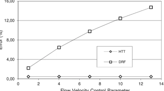
Figures 10 and 11 depict graphs which illustrate the numerical performance of both formulations as a function of the flow velocity, controlled through the parameter m. First of all, in Fig. 10, it is depicted the mean percentage error related to temperature numerical results along the horizontal direction. The performance of the HTT approach is undoubtedly superior to that of the DRF approach. HTT errors were quite low for the velocity range considered.
With respect to the numerical results for the heat flux on face 4, depicted in Fig. 11, the performance of the HTT approach was again superior, being practically insensitive to the variations of the flow velocity intensity for the velocity range considered. The mean percentage error is practically constant, around 0.471%.
Figure 10. Temperature percentage mean error along the horizontal direction versus flow velocity, for example 2.
Figure 11. Normal flux percentage mean error on face 4 versus flow velocity, for example 2.
Two-Dimensional Fluid Flow with Constant Velocity Field
In two-dimensional problems, the harmonic transformation requires a more restrict condition than irrotational fluid flow condition. This condition appears by considering Eqs. (13) and (14), that is:
1 1
exp( / K)
x x
∂ψ ∂θ
= −φ
∂ ∂ (34)
2 2
exp( / K)
x x
∂ψ ∂θ
= −φ
∂ ∂ (35)
Taking the cross derivatives of the former equations it is found:
2 1
1 2
v v
x x
∂θ ∂θ
=
∂ ∂ (36)
It means that a very limited number of two-dimensional problems can be solved by the proposed method. However, to show the good numerical performance of HTT this case study considers a two-dimensional heat transfer problem, in which the velocity field has constant components in the x and y directions. Essential boundary conditions are prescribed on the four sides of length L of a square control volume; the analytical solution of this case-study is:
(
x y)
K
1
v x v y
e
+θ =
(37)Figure 12 shows the physical and geometrical characteristics of the control volume of this problem. The horizontal and vertical components of the particle velocity vector are respectively denoted by vx e vy.
The evaluation of the performance of DRF, QDR and HTT formulations will be carried out through comparison of the numerical results obtained for the boundary fluxes with analytical values, the latter being given by:
(
x y)
K x
1
v x v y
v e
x K
+ ∂θ
=
∂ (38)
(
x y)
K y
1
v x v y
v e
y K
+ ∂θ=
∂ (39)
0,00 0,80 1,60 2,40 3,20
0 20 40 60 80 100 120 140 160
E
rr
o
r
(%
)
Number of Boundary Elements HTT
DRF
0,00 1,00 2,00 3,00 4,00
0 20 40 60 80 100 120 140 160
E
rr
o
r
(%
)
Number of Boundary Elements HTT
DRF
0,00 2,00 4,00 6,00 8,00
0 2 4 6 8 10 12 14
E
rr
o
r
(%
)
Flow Velocity Control Parameter HTT
DRF
0,00 4,00 8,00 12,00 16,00
0 2 4 6 8 10 12 14
E
rr
o
r
(%
)
Flow Velocity Control Parameter HTT
The criteria and formulas for error computation are the same used previously, given by Eq. (28) and (29).
Figure 12. Physical and geometrical characteristics for example 3.
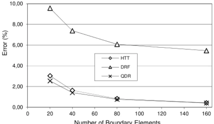
The first test carried out evaluates the behavior of the numerical solution versus the refinement of the boundary mesh used. The results presented in Fig. 13 correspond to fluxes on face 2, for Peclet number equal to 2. It is important to observe that fluxes on face two are more significant (higher and more prone to numerical error).
The graphs of Fig. 13 show again that HTT results approach the analytical solution as the mesh becomes finer and finer. The QDR results are superior to those obtained from the HTT formulation, as expected for low Peclet numbers. The results obtained with the DRF, shown in Fig. 13, are just acceptable, the lack of accuracy being due to the existence of boundary regions where results are not accurate at all. This lack of accuracy happens mainly over regions where the flux values are not dominant, as residuals of the interference of higher values of derivative elsewhere which are transmitted to other parts of the domain through the global interpolation inherent to the DRF. Anyway, results presented in Fig. 13 show the strong limitation of the DRF for some two-dimensional cases.
Figure 13. Normal flux percentage mean error on face 2 versus mesh refinement, for Peclet number equal to 2, for example 3.
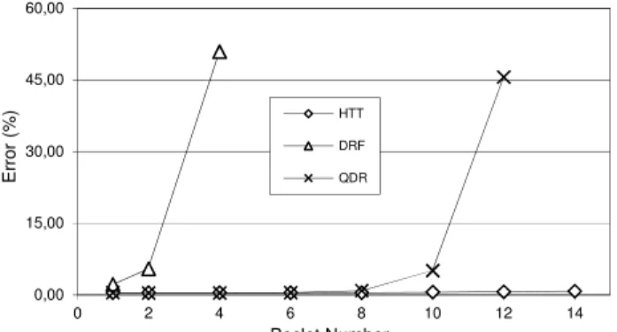
Next it is analyzed the performance of the three approaches (in what accuracy is concerned) for different Peclet numbers. A fixed mesh of 160 elements is employed, and the error of the flux on face two versus Peclet Number is plotted in Fig. 14.
The graphs depicted in Fig. 14 show that increasing the Peclet number a little causes complete failure of the DRF. Errors increase very quickly from Peclet number equal to two onwards. The QDR approach requires mesh refinement in order to yield acceptable accuracy for higher Peclet numbers; acceptable results are obtained for Peclet numbers lower than 10. For Peclet numbers in the interval [0,10] the HTT approach presented its best performance; the error
was under 1%. In fact, numerical experiments, not shown here, gave acceptable results for the HTT approach up to Peclet numbers equal to 20, for a fixed 160 boundary element mesh. Peclet numbers higher than 20 require a finer discretization.
Figure 14. Normal flux percentage mean error on face 2 versus Peclet number, for a mesh with 160 boundary elements, for example 3.
Conclusions
The formulation presented in this paper showed to be suitable and efficient to carry out numerical modeling of one-dimensional and of a special class of two-dimensional diffusive-advective problems. The HTT approach overcomes the difficulty inherent to the Dual Reciprocity Formulation and other similar approaches: the use of auxiliary radial basis interpolation functions with non-compact support. The HTT approach does not require domain interpolation, thereby, the solution algorithm is simpler to implement than those originated from de DRF, and is much cheaper as there is no need to invert matrices. For the case of the analysis with one hundred and sixty elements CPU time for a computer program based on the Harmonic Transformation Technique (HTT) is about 17% of the CPU time of a similar program based on Quasi-Dual Reciprocity (QDR) and is 24% of the CPU time of a computer program based on the traditional Dual Reciprocity Formulation (DFR). Besides, the proposed HTT approach manages to represent with the same accuracy small and high values of the boundary unknowns. Thus, the numerical solution is more stable and accurate, especially for higher Peclet numbers.
Results of the HTT approach showed to be quite good even in the case of a variable velocity field over the domain, despite the limited accuracy of the scheme used to integrate the transformation variable; it is important to notice that other formulations usually yield poor results in this case. Another advantage of the HTT is that the incompressibility condition is not required, whereas QDR only can be applied to potential fluid flow problems. Last, it must be highlighted that the HTT, such as the QDR formulation, does not require the use of poles to improve its accuracy, a necessary and expensive procedure required by DRF.
It is necessary to emphasize that the HTT performance can still be improved if high order boundary elements are employed. Naturally, every Boundary Element formulations would have better performance by increasing elements order, but for the HTT technique the improvement will be quite higher, because the accuracy of approximation scheme given by Eq. (17) is also related to the boundary element order.
The main problem of HTT is its limitation to one-dimensional and particular two-dimensional applications. However, as mentioned previously, in some transient problems it is interesting to implement simple and quick one-dimensional spatial model coupled with a robust time integration scheme to achieve response estimations or benchmarks. It must be also included some dynamic
y
x
L
face1
fa
c
e
2
vy vx
v L p
K
=
0,00 1,25 2,50 3,75 5,00
0 20 40 60 80 100 120 140 160
E
rr
o
r
(%
)
Number of Boundary Elements HTT DRF QDR
0,00 1,50 3,00 4,50 6,00
0 2 4 6 8 10
E
rr
o
r
(%
)
problems that have effective one dimensional wave propagation. For this purpose the HTT formulation is suitable: in addition to the high accuracy, mathematical simplicity and low computational cost, the computational code requests quite short and simple programming algorithms.
References
Batchelor, G.K., 1967, “An Introduction to Fluid Dynamics”, Cambridge University Press, New York, 660 p.
Bejan, A., 1993, “Heat Transfer”, John Wiley & Sons, New York, 676 p. Bennett, C.O., Myers, J.E., 1983, “Momentum, Heat, and Mass Transfer”, McGraw-Hill International Editions, Singapore, 832 p.
Brebbia, C.A., 1978, “The Boundary Element Method for Engineers”, Pentech Press, London, 188 p.
Brebbia, C.A., Telles, J.C. and Wrobel, L., 1984, “Boundary Element Techniques: Theory and Applications in Engineering”, Springer – Verlag, Berlin, 464 p.
Brebbia, C.A., Walker, S., 1980, “Boundary Element Techniques in Engineering”, Newnes-Buttterworths, U.K, 210 p.
Buhmann, M.D., 2003, “Radial Basis Functions: Theory and Implementations”, Cambridge University Press, 1ª ed., New York, 272 p.
Golberg, M.A., Chen, C.S., 1994, “The Theory of Radial Basis Functions applied to the BEM for Inhomogeneous Partial Differential equations”, BE Communication, Vol. 5, pp. 57-61.
Honna, T., Tanaka, Y. and Kaki, I., 1985, “Regular Boundary Element Solutions to Steady State Convection-Diffusion Equations”, Eng. Analysis with Boundary Elements, Vol. 2, pp. 95-99.
Incropera, F.P., Witt, D.P., 1992, “Fundaments of Heat and Mass Transfer” (in Portuguese) - Guanabara Koogan S.A., Rio de Janeiro, 584 p.
Karur, S.R., Ramachandran, P.A., 1994, “Radial Basis Function Approximation in the DualReciprocity Method”, Mathematical and Computer Modelling, Vol. 20, No. 7, pp. 59-70.
Loeffler, C.F., Dan, M.L., 2004, “Modeling of a Forced Convection Problem with Compressive Flow Through the Diffusive-Advective
Equation” (in Portuguese), Engineering, Science and Technological Journal, Federal University of Espírito Santo, Vol. 7, No. 5, pp. 21-25.
Loeffler, C.F., Mansur W.J., 2003, “Quasi-Dual Reciprocity Boundary Element Formulation for Incompressible Flow: Application to the Diffusive-Advective Equation”, International Journal for Numerical Methods in Engineering, Vol. 58, pp. 1167-1186.
Nardini, D., Brebbia, C.A., 1982, “A New Approach to Free Vibration Analysis using Boundary Elements”, Proceeding of the Fourth International Seminar, Boundary Element Methods in Engineering, Southampton.
Partridge, P.W., 1997, “Approximation Functions in the Dual Reciprocity Method”, International Journal of Boundary Elements Communications, Vol. 8, No. 1, pp. 1-4.
Partridge, P.W., Brebbia, C.A. and Wrobel, L.C., 1992, “The Dual Reciprocity Boundary Element Method”, Computational Mechanics Publications and Elsevier, London, 464 p.
Pasquetti, R., Caruso, A., 1990, “Boundary element approach for transient and non-linear thermal diffusion”, Num. Heat Transf., Part B, Vol. 17, pp. 83-99.
Ramachandran, P. A., 1994, “Boundary Element Methods in Transport Phenomena”, Computational Mechanics Publication and Elsevier Applied Science, London, 406 p.
Spitzer, K.H., Harste, K., Weber, B., Monheim, P. and Schewerdtfeger, K., 1992, “Mathematical Model for Thermal Tracking and On –Line Control in continuous Casting”, ISIJ international, Vol. 32, No. 7, pp. 848-856.
Sutradhar, A., Paulino, G.H. and Gray, L.J., 2002, “Transient heat conduction in homogeneous and non-homogeneous materials by the Laplace transform Galerkin boundary element method”, Engineering Analysis with Boundary Elements, Vol. 26, pp. 119-132.
White, F.M., 1986, “Fluid Mechanics”, McGraw-Hill-Kogakusha, Tokyo, 732 p.