Dejan Taniki
ć
[email protected] University of Belgarde Technical Faculty of Bor V.J. 12 19210 Bor, Serbia
Velibor Marinkovi
ć
[email protected] University of Niš Faculty of Mechanical Engineering A. Medvedeva 14, 18000 Niš, Serbia
Modelling and Optimization of the
Surface Roughness in the Dry
Turning of the Cold Rolled Alloyed
Steel Using Regression Analysis
Surface quality of the machined parts is one of the most important product quality indicators and one of the most frequent customer requirements. The average surface roughness (Ra) represents a measure of the surface quality, and it is mostly influenced by the following cutting parameters: the cutting speed, the feed rate, and the depth of cut. Quantifying the relationship between surface roughness and cutting parameters is a very important task. In this study regression analysis was used for modelling and optimization of the surface roughness in dry single-point turning of the alloyed steel, using coated tungsten carbide inserts. The experiment has been designed and carried out on the basis of a three-level full factorial design. The linear, the quadratic and the power (non-linear) mathematical models were selected for the analysis. Obtained results are in good accordance with the experimentally obtained data, confirming the effectiveness of regression analysis in modelling and optimization of surface roughness in the turning process. The general conclusion is that the surface roughness has a clear downward trend with the cutting speed increase and decrease in the feed rate and the depth of cut.
Keywords: turning, surface roughness, regression analysis, optimization
Introduction1
The key demands in the case of cutting technology include: reducing component size and weights, enhancing surface quality, tolerances and manufacturing accuracies, reducing costs and reducing batch sizes (Byrne, Dornfeld and Denkena, 2003).
The surface roughness of the machined parts is one of the most significant product quality characteristic. It is a key factor in evaluating the quality of a product and has the great importance on the functional behaviour of the machined parts in exploitation as well as manufacturing costs.
The lack of good surface quality fails to satisfy one of the most important technical requirements for mechanical products, while extremely high level of surface quality causes higher production costs and lower overall productivity of cutting operations.
The desired surface quality is a critical constraint in selecting the optimal cutting parameters in the production process (Jacobs, Jacob and Kochan, 1972; Silva, Saramago and Machado, 2009; Pasam et al., 2010). Hence, it is of great importance to quantify the relationship between surface roughness and cutting conditions. Tool wear phenomenon, studied by a large number of scientists, directly influences the quality of the machined surface (Rosa et al., 2010). The surface roughness also influences the tribological characteristics, the fatigue strength, the corrosion resistance and the aesthetic appearance of the machined parts.
On the other side, the surface finish in the turning process is influenced by a number of factors, such as: cutting speed, feed rate, depth of cut, material characteristics, tool geometry, stability and stiffness of the machine tool – cutting tool – workpiece system, built-up edge, cutting fluid, etc. Therefore, the ideal surface quality could not be achieved even in the ideal cutting and environmental conditions.
The surface roughness always refers to deviation from the nominal surface. The actual surface profile is the superposition of the errors of the form, waviness and roughness.
There are various parameters used to evaluate the surface roughness. In the present research the average surface roughness (Ra), also known as the Centerline Average (CLA), was selected for
Paper received 1 March 2011. Paper accepted 29 June 2011. Technical Editor: Anselmo Diniz
the characterization of the surface finish in the cutting process. It is the most widely used surface finish parameter in industry.
The turning process is one of the most fundamental among various cutting processes, and it is also the most applied metal removal operation in the real manufacturing environment.
In order to achieve the best possible surface roughness many machine tool operators rely on their own experience and/or the guidelines given in the machine tool manuals and handbooks. It has also been observed that experienced machine tool operators use trial-and-error approach, i.e. they estimate surface quality by visually comparing the actual surfaces on the machined part with those on the measuring calibrator.
Benardos and Vosniakos (2003) give a general review of predicting the surface roughness in machining. Also, a comprehensive overview of the optimization techniques in the metal cutting processes is presented by Mukherjee and Ray (2006). The determination of (near) optimal cutting conditions, using conventional and non-conventional optimization techniques, as well as in-process parameter relationship modelling, are described in detail.
Thangavel and Selladurai (2008) developed a mathematical model to study the effect of cutting parameters on the surface roughness using the response surface methodology (RSM). After the regression analysis and the variance analysis, it was found that the model is adequate and that all the main cutting parameters have a significant impact on the surface roughness.
Choudhury and El-Baradie (1997) utilized the same methodology in order to develop the surface roughness model in dry turning of high-strength steel. Also, Sahin and Motorcu (2005) employed RSM for predicting the surface roughness in turning of mild steel with the coated carbide tools.
Arbizu and Perez (2003) employed a classic experimental technique design to determine surface roughness in the turning process. The second-order mathematical model was adopted. It was observed that the feed rate and the depth of cut have negative influences on the average surface roughness (Ra), while there is an optimum cutting speed, which provides a minimum of the average surface roughness value.
values of the surface roughness are achieved when employing a PVD coated (TiAlN) insert instead of a CVD coated (TiCN+Al2O3+TiN) insert.
Davim (2001) and Davim et al. (2009) investigated the cutting parameter effects on the surface finish in steel turning using the design of the experiment and the artificial neural network. For the purpose of experimentation, the authors selected the standard L27(33) orthogonal array, based on the Taguchi experimental design. The multiple linear regression and the three-layer back-propagation neural network models were developed to study the effects of the cutting conditions on the surface roughness parameters (Ra and Rt). The good agreement exists between the experimental and predicted results obtained from these models.
In addition to the abovementioned, other methodologies are being employed for predicting the surface roughness, such as Taguchi method (Kopač, Bahor and Soković, 2002; Hascalic and
Caydas, 2008), artificial neural networks (Karayel, 2009; Özel and Karpat, 2005; Lu, 2008; Marinković and Tanikić, 2011),
neuro-fuzzy systems (Jiao et al., 2004; Kirby and Chen, 2007; Tanikić et
al., 2010), genetic algorithms (Chen and Chen, 2003; Cus and Balic, 2003), and artificial intelligence or soft computing techniques (Samanta, Erevelles and Omurtag, 2009).
Research in this paper refers to dry turning process. In general, machining without the use of any cutting fluid (coolant and lubricant) is nowadays popular due to the concern regarding the safety of the environment and the health protection (Sreejith and Ngoi, 2001), (Klocke and Eisenblaetter, 1997). Besides everything else, the implementation of dry machining includes: non-pollution of the atmosphere and no residue on the chip, which causes reduced disposal and cleaning costs. It is harmless to skin and it is allergy free. Moreover, it offers cost reduction in machining.
Nomenclature
a = depth of cut, mm
b = (k x 1) vector of the first-order regression coefficients B = (k x k) symmetric matrix, whose main diagonal elements
are the pure quadratic coefficients, while off-diagonal elements are one-half mixed quadratic coefficients b0 = free term (parameter) of the mathematical model
bi = linear terms
bii = quadratic terms
bij = interaction terms
f = feed rate, mm/rev R = correlation coefficient Ra = average surface roughness, µm
ai
Rˆ = predicted average surface roughness, µm V = cutting speed, m/min
{wi} = canonical independent variables (factors)
x = (k x 1) vector of the independent variables xi = coded variables (factors)
Xi = natural variables
y = estimated response Y = estimated natural response ye = measured response
Greek Symbols
δi = absolute percentage error, % ε = experimental error
{λi} = eigenvalues (canonical coefficients)
Experimental Work
The parameters (factors) considered in the present paper are: the cutting speed (V), the feed rate (f) and the depth of cut (a). The
average surface roughness (Ra) was chosen for a target function (response, output). Since it is obvious that the effects of the factors are non-linear, an experiment with factors at three levels was set up (Table 1).
Table 1. Cutting factors and their levels.
Cutting factor Symbol Unit
Factor levels Level 1
(Low)
Level 2 (Middle)
Level 3 (High) Cutting speed V (X1) (m/min) 80 110 140
Feed rate f (X2) (mm/rev) 0.071 0.196 0.321 Depth of cut a (X3) (mm) 0.5 1.125 2.0
The factor ranges were chosen with different criteria for each factor, aiming at the widest possible range of values, in order to have a better utilization of the proposed models. At the same time, the characteristics of the mechanical system and manufacturer's recommendations are taken into account.
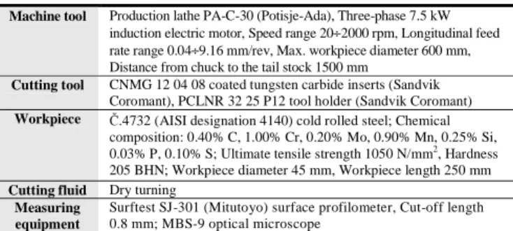
Table 2. Machining system, workpiece and measuring equipment.
Production conditions used in the experiment are shown in Table 2. All of the trials have been conducted on the same machine tool, with the same cutting tool type and the same other cutting conditions. Measuring equipment and surface roughness report are shown in Fig. 1.
Figure 1. Measuring equipment (a) and surface roughness report (b).
Profile of the machined surface for different cutting regimes is presented in Fig. 2. Part of the experimental results, which refers to the surface finish in the single-point turning process, is analysed in this study.
Machine tool Production lathe PA-C-30 (Potisje-Ada), Three-phase 7.5 kW induction electric motor, Speed range 20÷2000 rpm, Longitudinal feed rate range 0.04÷9.16 mm/rev, Max. workpiece diameter 600 mm, Distance from chuck to the tail stock 1500 mm
Cutting tool CNMG 12 04 08 coated tungsten carbide inserts (Sandvik Coromant), PCLNR 32 25 P12 tool holder (Sandvik Coromant) Workpiece Č.4732 (AISI designation 4140) cold rolled steel; Chemical
composition: 0.40% C, 1.00% Cr, 0.20% Mo, 0.90% Mn, 0.25% Si, 0.03% P, 0.10% S; Ultimate tensile strength 1050 N/mm2, Hardness
205 BHN; Workpiece diameter 45 mm, Workpiece length 250 mm Cutting fluid Dry turning
Measuring equipment
Figure 2. Profile of the machined surface for cutting regimes: a) V = 110 m/min, a = 1.25 mm, f = 0.321 mm/rev b) V = 110 m/min, a = 1.25 mm, f = 0.196 mm/rev c) V = 110 m/min, a = 1.25 mm, f = 0.071 mm/rev
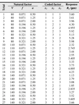
A design matrix was constructed on the basis of the selected factors and factor levels (Table 3). The method of coding the cutting factors is explained in the following chapter.
Table 3. Experimental design and results.
T
ri
a
l Natural factor Coded factor Response
Ra (µµµµm)
V f a x1 x2 x3
1 80 0.071 0.50 1 1 1 3.60 2 80 0.071 1.25 1 1 2 3.61 3 80 0.071 2.00 1 1 3 3.96 4 80 0.196 0.50 1 2 1 4.30 5 80 0.196 1.25 1 2 2 4.955 6 80 0.196 2.00 1 2 3 5.92 7 80 0.321 0.50 1 3 1 5.13 8 80 0.321 1.25 1 3 2 5.28 9 80 0.321 2.00 1 3 3 5.98 10 110 0.071 0.50 2 1 1 2.32 11 110 0.071 1.25 2 1 2 2.745 12 110 0.071 2.00 2 1 3 3.44 13 110 0.196 0.50 2 2 1 2.55 14 110 0.196 1.25 2 2 2 3.405 15 110 0.196 2.00 2 2 3 3.33 16 110 0.321 0.50 2 3 1 3.73 17 110 0.321 1.25 2 3 2 4.005 18 110 0.321 2.00 2 3 3 4.23 19 140 0.071 0.50 3 1 1 1.13 20 140 0.071 1.25 3 1 2 2.79 21 140 0.071 2.00 3 1 3 3.08 22 140 0.196 0.50 3 2 1 1.85 23 140 0.196 1.25 3 2 2 2.835 24 140 0.196 2.00 3 2 3 3.27 25 140 0.321 0.50 3 3 1 3.52 26 140 0.321 1.25 3 3 2 3.605 27 140 0.321 2.00 3 3 3 3.66
The selected design matrix was a full factorial design consisting of 27 rows of coded/natural factors, corresponding to a number of trials. This design provides a uniform distribution of experimental points within the selected experimental hyper-space and the experiment with high resolution. The experiment was conducted using a new set of coated tungsten carbide inserts, preventing possible mistakes caused by using a worn tool. The average surface roughness values (Ra), shown in Table 3, are the average values of three measurements.
Regression Analysis
Brief overview
The cutting processes based on the formation and removing chips from the workpiece surface are very complex and still incompletely explored phenomenon.
The extraordinary complexity of the mechanical, tribological, and thermodynamical phenomena in the cutting zone does not allow to determine a reliable and comprehensive theoretical model, which could explain the essence and the mechanism of chip formation and the shaping of surface roughness.
The theoretical approach is always based on simplifications and idealizations. It does not take into account any imperfections of the
cutting process and neglects the effects of many process factors, as well as environment factors (noise).
Hence, various theoretical models that have been proposed are not accurate enough and can be applied only to a limited range of processes and cutting conditions. For these reasons, most researchers mainly use the empirical research.
The regression analysis technique, based on the experimental data, is a powerful tool for modelling and analysing real processes, whose nature and behaviour cannot be explained using a theoretical approach. Many researchers use this method successfully in various fields.
Therefore, with the efficient regression analysis researchers cannot only rely on their perspicacity and intuition, but must have a relevant knowledge of the researched phenomenon and the experimental techniques.
Many experiments involve studying the effects of more factors. In these cases, generally, the design of experiment (DoE) is the most efficient type of experiment, especially in relation to the traditional one-factor-at-a-time experiment. The selection of a proper experimental design is essential for reducing the experimental cost and time.
The success of a regression analysis depends largely on the choice of appropriate mathematical models. Many studies have shown that the choice of mathematical models in the form of polynomials provides the most appropriate and effective approximation of the experimental data. These are the following mathematical models:
a) linear mathematical model
∑
= + = − = k i i ie b b x
y y
1 0
ε (1a)
b) quasi-linear mathematical model
∑ ∑
∑
− = =+ = + + = − = 1 1 1 1 0 k i k i j j i ij k i i ie b bx b xx
y
y ε (1b)
c) non-linear (quadratic) mathematical model
∑∑
∑
∑
− = =+ = = + + + = − = 1 1 1 1 2 1 0 k i k i j j i ij k i i ii k i i ie b bx b x b xx
y
y ε (1c)
where y is the estimated response, ye is the measured response, ε is the independent random variable (experimental error), normally distributed with a mean of zero and a constant variance of σ2
, b0 is the free term (parameter) of the mathematical model, bi are the linear terms, bii are the quadratic terms, bij are the interaction terms, and k is the number of the independent variables (factors). The parameters of the mathematical model can only be statistically estimated on the bases of the experimental results.
The relationship between dependent variable (response) and independent variables (factors) can also be expressed in the form of the multiple power function:
∏
= = = k i b i b k bb X X k c X i
X c Y 1 0 2 1
0 1 2.... (2a)
Applying the logarithmic transformation, the non-linear equation (2a) can be converted into the following linear equation:
∑
= + = + + + = k i i i kk X c b X
b X b c Y 1 0 1 1
0 ln ... ln ln ln
ln
ln (2b)
When the variables in logarithmic scale in Eq. (2b) are replaced with the new variables, y = lnY, xi = lnXi (b0 = lnc0), then it can be rewritten in a linear form, defined by Eq. (1a). If the multiple power function includes first-order factor interactions, then Eq. (2b) represents the quasi-linear mathematical model, defined by Eq. (1b). But, in this particular case, it is not necessary (Marinković and
Lazarević, 2010).
In general, the mathematical models may also include higher-order factor interactions. Since the impact of higher-higher-order factor interactions is usually negligible, these terms of the mathematical model may be omitted. On the other hand, in many cases, adding the high-order polynomial terms does not really improve the fit, but increases the complexity of the mathematical model. Thus, it is useful to try fitting using a lowest-order polynomial that adequately describes the system/process.
The statistical method often used to estimate the unknown parameters in a mathematical model is the method of least squares.
The number of factor levels within the selected range is theoretically arbitrary, whereas practice confirms that it is sufficient to choose: two levels for (quasi) linear mathematical model, and three levels for non-linear (quadratic) mathematical model.
Since input factors may be various physical values (temperature, pressure, volume, velocity, etc.) it is useful to perform their coding. There are two ways of coding the independent variables (factors) on three levels. It is accomplished by means of the transforming equations:
a) for levels (–1 , 0, +1):
) , 1 ( ; 1 2 min max
min i k
X X X X x i i i i
i − − =
−
= (3a)
b) for levels (1, 2, 3):
) , 1 ( ; 1 2 min max
min i k
X X X X x i i i i
i − + =
−
= (3b)
where xi are coded variables (factors), Xi are natural variables, from
Ximax to Ximin, in the design factor space of interest to the experimenter, Ximax and Ximin are the highest and the lowest values of the natural variables Xi respectively, and k is the number of the input factors.
The most useful application for DoE is to optimize a process/system. The process optimization is assured by minimizing or maximizing an objective function regarding the given (in)equality constraints. The second-order mathematical model may be written in matrix notation as following (Montgomery, 2001):
Bx x' b x' +
+ =ˆ0 ˆ b
y (4)
where x is a (k x 1) vector of the independent variables, b is a (k x 1) vector of the first – order regression coefficients and B is a (k x k) symmetric matrix whose main diagonal elements are the pure quadratic coefficients, while off-diagonal elements are one-half mixed quadratic coefficients.
The stationary (optimal) point is obtained from the following relation:
b B
x0 1
2 1
-−
= (5)
Thereby it implies that the optimum conditions of objective function are met.
Furthermore, by substituting Eq. (5) into Eq. (4) the predicted response at the optimal point can be found as:
b x'0 0 0 2 1 ˆ ˆ =b +
y (6)
For the characterization of the surface response (output) it is necessary to translate the selected mathematical model into a canonical form. Canonical transformation transfers the origin in the stationary point and rotates the coordinate axis to match with the main axes of the fitted surface response.
Canonical form of quadratic mathematical model can be expressed as follows:
∑
= = − k i i iw y y 1 2 0 ˆˆ λ (7)
where {wi} are the canonical independent variables (factors) and {λi} are their eigenvalues (canonical coefficients).
Canonical coefficients are the roots of the characteristic equation:
0 = − I
B λ (8)
Checking the correctness of calculation is done according to:
∑
∑
= = = k i k i ii i b 1 1λ (9)
Canonical equations contain no linear effects or interactions, which makes them more suitable for the analysis of the surface response. The geometric form of the response surfaces is determined by the stationary point, algebraic signs, and magnitudes of their own values (Novik and Arsov, 1980).
If the eigenvalues are all negative, the response surface has a maximum; if they are all positive, the response surface has a minimum; if they have mixed signs, the response surface has a saddle point.
At least one eigenvalue equal to zero (or close to zero) indicates the presence of a "ridge" in the response surface.
It should be noted that optimization of the real system/process makes sense in a limited space of independent variables (factors). The constraints, in terms of the coded variables, are most common specified in the form of (in)equations as:
) , 1 ( ; max
min x x i k
xi ≤ i≤ i = (10)
where ximin and ximax are the lowest and the highest values of the independent variables xi, respectively.
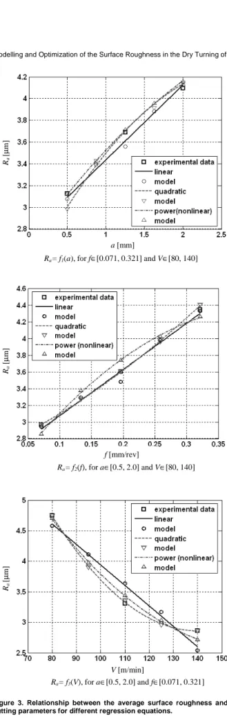
Figure 3. Relationship between the average surface roughness and the cutting parameters for different regression equations.
Application of the regression analysis
The linear, the quadratic and the non-linear mathematical models were selected for the analysis in this paper. The parameters of Eq. (1a), Eq. (1c), and Eq. (2b) have been estimated by means of the least-square method, using Matlab software package. In this way, the following multiple regression equations were obtained:
3 2
1 0.6925 0.4856 9442
. 0 1704 . 3
ˆ x x x
y= − + + (11a)
3 2 3
1 2
1 2
3
2 2 2
1 3
2 1
1617 . 0 0567 . 0 1196 . 0 0811 . 0
0547 . 0 4981 . 0 02 . 1 0361 . 1 8106 . 2 8443 . 3 ˆ
x x x
x x
x x
x x
x x x
y
− +
− −
− +
+ + +
− =
(11b)
3 2
1 0.2647 0.2393 9835
. 0 2950 . 6
ˆ x x x
y= − + + (11c)
The coding of the process factors was carried out according to the Eq. (3b). The fitted multiple regression equations in terms of the natural levels of the cutting speed, the feed rate, and the depth of cut may be obtained by substituting the transforming Eq. (3b) into the Eq. (11). These equations are not presented in this paper.
The graphs from Fig. 3 clearly show that the quadratic mathematical model most accurately approximates the experimental results.
The preliminary information of the quantitative and qualitative impact on the objective function (response) of each individual factor in the regression equations can be obtained from its parameters sign and magnitude. The negative sign for the parameter of the cutting speed shows that the surface roughness improves with the increase in the cutting speed. The positive sign for the parameters of the feed rate and the depth of cut indicates that the surface roughness deteriorates with the increase in these two factors. Furthermore, the given regression equation and Pareto chart (Fig. 4) suggest that the dominant process factor is the cutting speed, while the effects of the feed rate and the depth of cut are considerably smaller. The factor interactions have the least influence on the considered problem. In order to take into account the contribution from the factor interactions, these terms were not neglected.
Figure 4. Pareto chart.
The criterion used to estimate the efficiency and ability of the mathematical model to predict average surface roughness could be the absolute percentage error – δi, which is defined by equation:
Ra= f3(V), for a∈[0.5, 2.0] and f∈[0.071, 0.321]
Ra
[
µ
m
]
V [m/min]
Ra= f1(a), for f∈[0.071, 0.321] and V∈[80, 140]
Ra
[
µ
m
]
a [mm]
Ra= f2(f), for a∈[0.5, 2.0] and V∈[80, 140]
Ra
[
µ
m
]
f [mm/rev]
V
f
a
V2
f x a
V x f
a2
V x a
f2
(%) 100 ˆ
ai ai ai i
R R
R −
=
δ (12)
where Rˆ and ai R represent the predicted and measured average ai
surface roughness for i-th trial, respectively.
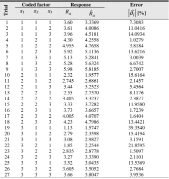
The average surface roughness calculated according to the Eq. (11b), and errors calculated according to the Eq. (12) are given in Table 4.
Table 4. Experimental and predicted results and absolute percentage error.
T
ri
a
l Coded factor Response Error
i
δ [%]
x1 x2 x3 Ra
a
Rˆ
1 1 1 1 3.60 3.3369 7.3083
2 1 1 2 3.61 4.0086 11.0416 3 1 1 3 3.96 4.5181 14.0934
4 1 2 1 4.30 4.2558 1.0279
5 1 2 2 4.955 4.7658 3.8184 6 1 2 3 5.92 5.1136 13.6216
7 1 3 1 5.13 5.2841 3.0039
8 1 3 2 5.28 5.6324 6.6742
9 1 3 3 5.98 5.8185 2.7007
10 2 1 1 2.32 1.9577 15.6164 11 2 1 2 2.745 2.6861 2.1457 12 2 1 3 3.44 3.2523 5.4564 13 2 2 1 2.55 2.7570 8.1176 14 2 2 2 3.405 3.3237 2.3877 15 2 2 3 3.33 3.7282 11.9580 16 2 3 1 3.73 3.6657 1.7239 17 2 3 2 4.005 4.0707 1.6404 18 2 3 3 4.23 4.7986 13.4421 19 3 1 1 1.13 1.5747 39.3540 20 3 1 2 2.79 2.3598 15.4194 21 3 1 3 3.08 2.9827 3.1591 22 3 2 1 1.85 2.2544 21.8595 23 3 2 2 2.835 2.8778 1.5097 24 3 2 3 3.27 3.3390 2.1101 25 3 3 1 3.52 3.0435 13.5369 26 3 3 2 3.605 3.5052 2.7684 27 3 3 3 3.66 3.8047 3.9536
The mean absolute percentage error |δ|=8.50
[ ]
%Figure 5. Performance of the quadratic mathematical model.
The accuracy of any empirical model can also be done by means of statistical parameters, for example, correlation coefficient. The correlation coefficient (R) is a statistical measure of the strength of correlation between the predicted and measured values. For the current problem, the following result is obtained: R = 0.956 (Fig. 5).
Figure 6. Effects of the cutting parameters on the surface roughness.
Similar results were obtained by other researchers (Thangavel and Selladurai, 2008), for similar cutting conditions. The surface quality in turning is very sensitive to any change in cutting conditions. For example, changing of the cutting tool produces a different surface roughness even when all the other cutting conditions remain the same (Cakir, Ensarioglu and Demirayak, 2009).
Ra measured [µm]
R
a
p
re
d
ic
te
d
[
µ
m
]
a=0.5 [mm]
f [mm/rev] V [m/min]
Ra
[
µ
m
]
a=1.25 [mm]
f [mm/rev] V [m/min]
Ra
[
µ
m
]
a=2.0 [mm]
f [mm/rev] V [m/min]
Ra
[
µ
m
The optimization problem for the given turning process can be mathematically stated as follows: find the vector of cutting
factorsx0′ =(x1,x2,x3)∈R3, which minimizes the objective function
) , , ( ˆ f x1 x2 x3
y= (Eq. (11b)) subjected to 1≤xi≤3.
The surface roughness may continuously improve with the increase in the cutting speed, up to certain level. Beyond this critical level, further increase in the cutting speed will deteriorate the surface roughness (Sundaram and Lambert, 1981). Therefore, in many cases there is an optimal value of the cutting speed, which provides a minimum value of the surface roughness. It is confirmed by the results of research of many authors (Arbizu and Perez, 2003; Karayel, 2009).
In this particular case, Eq. (5) and Eq. (6) give:
) 5488 . 5 , 6918 . 1 , 7086 . 3 ( 0= ′
x , yˆ0=3.744.
Obviously, the optimal point is outside of the given experimental space. From Fig. 3 and Fig. 6, it can be concluded that the surface roughness has a clear downward trend with the cutting speed increase and decrease in the feed rate and the depth of cut. It can be shown that there is no global optimum in this case, i.e. this is the so called ridge system.
When it comes to optimization problem with constraints, the conditional optimum is located at one of the corresponding boundary of ranges of cutting factors.
According to the above described procedure, translating the coded in the natural factors gives: X0′ =(136.4,0.071,0.5),
568 . 1 ˆ ˆ
0 0≡Ra =
Y .
By using Eq. (8), the following eigenvalues are obtained:
) 08 . 0 , 51 . 0 , 12 . 0 (−
=
i
λ . These eigenvalues satisfy Eq. (9). Also, 0
3≈
λ indicates that the considered system is really a ridge system.
Conclusion
The aim of this work was to investigate the effects of the cutting parameters (the cutting speed, the feed rate and the depth of cut) on the average surface roughness, during the dry turning of the alloy steel, using coated tungsten carbide inserts. The dry turning is safe for the environment (atmosphere, water) and health as well as cheaper. Therefore, it is useful to analyse the effect of cutting conditions on the surface quality in dry turning.
In the first phase of this work, surface roughness was measured using the surface profilometer, which gives a relatively good indication of the measured roughness. The relationships among the inputs and corresponding outputs are established from the measured data, as well as the trends of surface roughness changing with cutting regimes changes.
The modelling and the optimization of the experimentally obtained data were performed using the regression analysis. In general, the results of the modelling are in good agreement with the experimentally obtained data.
References
Arbizu, I.P., and Perez, C.J.L., 2003, "Surface Roughness Prediction by Factorial Design of Experiments in Turning Processes", Journal of Materials
Processing Technology, Vol. 143-144, pp. 390-396.
Benardos, P.G., and Vosniakos, G.-C., 2003, "Predicting Surface Roughness in Machining: a Review", International Journal of Machine
Tools and Manufacture, Vol. 43, Iss.8, pp. 833-844.
Byrne, G., Dornfeld, D., and Denkena, B., 2003, "Advancing Cutting Technology", CIRP Annals – Manufacturing Technology, Vol. 52, No. 2, pp. 483-507.
Cakir, M.C., Ensarioglu, C., and Demirayak, I., 2009, "Mathematical Modeling of Surface Roughness for Evaluating the Effects of Cutting Parameters and Coating Material", Journal of Materials Processing
Technology, Vol. 209, No. 1, pp. 102-109.
Chen, M.-C., and Chen, K.-Y., 2003, "Optimization of Multipass Turning Operations with Genetic Algorithms: a Note", International Journal
of Production Research, Vol. 41, No. 14, pp. 3385-3388.
Choudhury, I.A. and El-Baradie M.A., 1997, "Surface Roughness Prediction in the Turning of High-strength Steel by Factorial Design of Experiment", Journal of Materials Processing Technology, Vol. 67, Iss. 1-3, pp. 55-61
Cus, F., and Balic, J., 2003, "Optimization of Cutting Process by GA Approach", Robotics and Computer Integrated Manufacturing, Vol. 19, Iss. 1-2, pp. 113-121.
Davim, J.P., 2001, "A Note on the Determination of Optimal Cutting Conditions for Surface Finish Obtained in Turning Using Design of Experiments", Journal of Materials Processing Technology, Vol. 116, Iss. 2-3, pp. 305-308.
Davim, J.P., Gaitonde, V.N., and Karnik, S.R., 2009, "Investigations Into the Effect of Cutting Conditions on Surface Roughness in Turning of Free Machining Steel by ANN Models", Journal of Materials Processing
Technology, Vol. 205, Iss. 1-3, pp. 16-23.
Hascalic, A., and Caydas, U., 2008, "Optimization of Turning Parameters for Surface Roughness and Tool Life Based on the Taguchi Method", International Journal of Advanced Manufacturing Technology, Vol. 38, No. 9-10, pp. 896-903
Jacobs, H.J., Jacob, E., and Kochan, D., 1972, "Spanungs-optimierung" (in German), VEB Verlag Technik, Berlin, Germany, 62 p.
Jiao, Y., Shuting L., Pei Z.J., and Lee E.S., 2004, "Fuzzy Adaptive Networks in Machining Process Modeling: Surface Roughness Prediction for Turning Operations", International Journal of Manufacturing
Research, Vol. 44, Iss. 15, pp. 1643-1651.
Karayel, D., 2009, "Prediction and Control of Surface Roughness in CNC Lathe Using Artificial Neural Network", Journal of Materials
Processing Technology, Vol. 209, Iss. 7, pp. 3125-3137.
Kirby, E.D., and Chen, J.C., 2007, "Development of a Fuzzy-Nets-Based Surface Roughness Prediction System in Turning Operations",
Computers & Industrial Engineering, Vol. 53, Iss. 1, pp. 30-42.
Klocke, F., and Eisenblaetter, G., 1997, "Dry Cutting", CIRP Annals –
Manufacturing Technology, Vol. 46, Iss. 2, pp. 519-526.
Kopač, J., Bahor, M., and Soković, M., 2002, "Optimal Machining
Parameters for Achiving the Desired Surface Roughness in Fine Turning of Cold Pre-formed Steel Workpieces", International Journal of Machine Tools
and Manufacture, Vol. 42, Iss. 6, pp. 707-716.
Lazarević, A., Marinković, V., and Lazarević D., 2010, “Expanded
non-linear mathematical models in the theory of experimental design: a case study”, 10th International Conference ″Research and Development in
Mechanical Industry″-RaDMI 2010, D. Milanovac, pp. 304-311.
Lu, C., 2008, "Study on Prediction of Surface Quality in Machining Process", Journal of Material Processing Technology, Vol. 205, Iss. 1-3, pp. 439-450.
Marinković, V., and Tanikić, D., 2011, "Prediction of the Average Surface
Roughness in dry Turning of Cold Rolled Alloy Steel by Artificial Neural Network", Facta Universitatis, Series: Mechanical Engineering, (in press).
Montgomery, D.C., 2001, "Design and Analysis of Experiments", John Wiley & Sons, New York, USA, 437 p.
Mukherjee, I., and Ray, P.K., 2006, "A Review of Optimization Techniques in Metal Cutting Processes", Computer and Industrial
Engineering, Vol. 50, Iss. 1-2, pp. 15-34.
Novik, F.S., and Arsov, J.B., 1980, "Optimization of Technological Processes by Experimental Design Method" (in Russian), Mashinostroenie/Technika, Moscow, Russia, 257 p.
Özel, T., and Karpat, Y., 2005, "Predictive Modeling of Surface Roughness and Tool Wear in Hard Turning Using Regression and Neural Networks", International Journal of Machine Tools and Manufacture, Vol. 45, Iss. 4-5, pp. 467-479.
Pasam, V.K., Battula, S.B., Madar Valli, P., and Swapna, M., 2010, "Optimizing Surface Finish in WEDM Using the Taguchi Parameter Design Method", Journal of the Brazilian Society of Mechanical Sciences and
Engineering, Vol. 32, No. 2, pp. 107-113.
Content", Journal of the Brazilian Society of Mechanical Sciences and
Engineering, Vol. 32, No. 3, pp. 234-240.
Sahin, Y., and Motorcu, A.R., 2005, "Surface Rougness Model for Machining Mild Steel with Coated Carbide Tool", Materials & Design, Vol. 26, Iss. 4, pp. 321-326.
Samanta, B., Erevelles, W., and Omurtag, Y., 2009, "Prediction of Workpiece Surface Roughness Using Soft Computing", Proc. Imech E. Part B: Journal of Engineering Manufacture, Vol. 222, No. 10, pp. 1221-1232.
Silva, J.D., Saramago, S. de F.P. and Machado, Á.R., 2009, "Optimization of the Cutting Conditions (Vc, fz and doc) for Burr Minimization in Face Milling of Mould Steel", Journal of the Brazilian Society of Mechanical
Sciences and Engineering, Vol. 31, No. 2, pp. 151-160.
Sreejith, P.S., and Ngoi, B.K.A., 2001, "Dry Machining: Machining of the Future", Journal of Materials Processing Technology, Vol. 101, Iss. 1-3, pp. 287-291.
Sundaram, R.M., and Lambert, B.K., 1981, "Mathematical Models to Predict Surface Finish in Fine Turning of Steel Part I", International Journal
of Production Research, Vol. 19, Iss. 5, pp. 547-556.
Tanikić, D., Manić, M., Devedžić, G., and Stević, Z., 2010, "Modelling
Metal Cutting Parameters Using Intelligent Techniques", Journal of
Mechanical Engineering, Vol. 56, No. 1, pp. 52-62.
Thangavel, P., and Selladurai, V., 2008, "An Experimental Investigation on the Effect of Turning Parameters on Surface Roughness", International