Parviz Ghadimi
[email protected] Amirkabir University of Technology Department of Marine Technology Tehran, IranMohammad Farsi
[email protected] Amirkabir University of Technology Department of Marine Technology Tehran, IranAbbas Dashtimanesh
[email protected] Amirkabir University of Technology Department of Marine Technology Tehran, IranStudy of Various Numerical Aspects
of 3D-SPH for Simulation of the Dam
Break Problem
Recently, the Smoothed Particle Hydrodynamics (SPH) method has been utilized as an effective tool for capturing details of the fluid flows. The Lagrangian nature of the SPH method facilitates the modeling of the free surface flows. In the present article, different numerical features of 3D-SPH are probed to find a set of options that can be used to achieve an accurate numerical simulation of the dam break problem. Several numerical techniques such as time stepping algorithm, filter density and viscosity treatment are considered as compiling options. Twelve sets of mentioned schemes are also chosen and the elevation of free surface flow is captured. The obtained results are compared against the experimental data existing in the literature. Finally, it is concluded that the Symplectic algorithm in conjunction with density filter and SPS turbulence model can be used to achieve the desired accurate numerical results.
Keywords: SPH, dam break, free surface flows, numerical aspects
Introduction1
Common problems in naval hydrodynamics and coastal engineering are comprised in studies of complicated free surface flows phenomena. Different methods have been implemented for the simulation of violent free surface motion. Possible algorithms of solutions can be based on fixed or moving grid solver of fluid dynamics equations coupled with techniques to capture the interface evolution (Kaceniauskas (2008); Del Pin et al. (2007); Kleefsman (2005); Lohner et al.(2007)). The computational drawback of the grid-based numerical methods is that they are very intricate in regrinding process and simulating breaking waves. Therefore, an alternative technique may be meshless methods. The smoothed particle hydrodynamics can be a good alternative to modeling violent free surface evolution because of its Lagrangian nature and other efficient characteristics. For example, no constraints are imposed on the geometry of the system and the initial conditions can be easily programmed without the need of complicated gridding algorithms.
Review papers by Benz (1998) and Monaghan (1982) cover the early development of SPH method. SPH was first applied thirty years ago to solve astrophysical problems by Lucy (1977) and Gingold and Monaghan (1977), since the collective movement of those particles is similar to the movement of a fluid and it can be modeled by the governing equations of the classical Newtonian hydrodynamics. This method uses integral interpolation theory and transforms the partial differential equations into an integral form. Furthermore, Smoothed Particle Hydrodynamics is a meshfree, Lagrangian, particle method for modeling fluid flows. Accordingly, this method is a very powerful tool that has been applied to a large range of industrial and environmental fluid flows (Monaghan and Kos (1999); Dalrymple and Rogers (2004); Rogers and Dalrymple (2006); Colagrossi and Landrini (2003)).
Multi-phase flows are also studied by Monaghan and Kocharyan (1995) using SPH. The SPH simulation of the free surface flows was also considered by some other researchers (Monaghan (1994) and Monaghan et al. (2000)). Panizzo and Dalrymple (2004) studied the wave which was generated by the underwater landslide. The impact of a single wave generated by a dam break with a tall
Paper received 28 January 2012. Paper accepted 14 August 2012 Technical Editor: Francisco Cunha
structure was modeled by Gomez-Gesteira and Dalrymple (2004). They used a three dimensional version of SPH. Shao and Gotoh (2004) analyzed the interaction between waves and a floating curtain wall attached to the bottom. Lee et al. (2006) studied the run up of SPH wave on a coastal structure. Crespo et al. (2008) developed a general purpose SPH code for solving two and three dimensional problems.
The aim of this paper is the analysis of dam break flows by considering various numerical aspects of smoothed particle hydrodynamics, such as time stepping algorithm, density filter and viscosity treatment. The dam break problem was first introduced by Stoker (1957). The problem consists of having an enclosed space filled with water. The barrier to one side is then removed and the water can freely flow into the void. For this purpose, a 3D-SPH code (3D-Sphysics) is used. The dam break is simulated with different combinations of mentioned compiling options and the results from the SPH method are compared with the experimental data in order to find the suitable combination that provides the best accuracy for the simulation. The experiment was performed by Kleefsman et al. (2005) in the maritime research institute Netherlands (MARIN).
After describing the SPH formulation, the governing equations are presented and subsequently various numerical aspects of SPH, studied in this article, are surveyed. The obtained results are also shown and, from the accuracy point of view, the best set of numerical techniques for simulation of the dam break problem is introduced. Finally, a brief conclusion is presented.
SPH Formulation
Integral representation of a function
The SPH formulation may be considered in two steps. The integral representation or the kernel approximation of field functions can be mentioned as a first part and the second part includes the particle approximation.
point or particle. The concept of integral representation of a function
( ) used in the SPH method starts from the following identity:
( ) = ( ) ( − ) (1)
where Ω is the volume of the integral that contains x. Also, ( ) is a function of the three-dimensional position vector of x, and ( −
′) is the Dirac delta function given by
( − ) = 10 =≠ (2)
In the SPH formulation, the Delta function ( − ′) is substituted by a smoothing function ( − ′, ℎ). Therefore, the integral representation of ( ) becomes
( ) = ( ) ( − , ℎ) (3)
In the current study, cubic spline is used as a kernel function and is given by
( , ℎ) =
1 −32 +34 # 0 ≤ ≤ 1
1
4 (2 − )# 1 ≤ ≤ 2 0 ≥ 2
(4)
where is '(&) in three dimensions.
Particle approximation
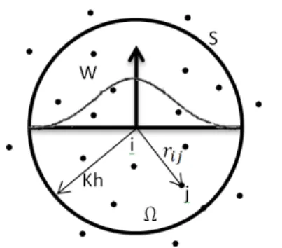
In the SPH method, the computational domain is approximated by a limited number of particles which are characterized as individual mass and space. The continuous integral can be converted to discretized forms of summation over all the particles in the support domain, as shown in Fig. 1. It may be concluded that the function ( ) can be written in the following form of discretized particle approximation:
( ) = *+-,
, .,/ ( − ,, ℎ) 0
,1&
(5)
where +, and -, represent the mass and density of the j-th particle, respectively.
Figure 1. Particle approximations using particles within the support domain of the smoothing function W for particle i.
Governing Equations
Three fundamental physical laws of conservation are the basic governing equations of the fluid dynamics which are as follows:
1. conservation of mass 2. conservation of momentum 3. conservation of energy
For this problem, conservation of mass and momentum must be used.
In the SPH formulation, the derivative of the density for particle i must be determined based on the continuity equation:
2-3
24 = * +,53,677 3, 36 0
,1&
(6)
where the sum extends over all neighboring particles and is the smoothing kernel evaluated at the distance between particles i and j.
The velocity can be updated by the momentum equation:
2538
24 = * +,(93
86
-3 + 9,86
-, ) 7 3,
7 36
0
,1&
(7)
Numerical Aspects of SPH
Viscosity treatment
To consider the diffusion term in the momentum equation, two different ways of 1) artificial viscosity and 2) laminar viscosity in addition to Sub-Particle Scale (SPC) turbulence, are investigated.
Artificial viscosity
Based on the work done by Monaghan (1992), by introducing the artificial viscosity, the momentum conservation equation can be written as
5:;
4 = − * +< <=>-<<+-?;;+ Π;<A ∇CCCC:; ;<+ D: (8)
where D: = (0, 0, −9.81) +HI is the gravitational acceleration. Therefore, the pressure gradient term in symmetrical form is also expressed in SPH notation as
J−1- ∇CC:?K
;= − * +<=
><
-<+
?;
-;∇CCCC:A ∇; CCCC:; ;< <
(9)
where ?L and -L are the pressure and density corresponding to the particle k. The viscosity term, M;<, can also be presented as
M;<= N−
O;<
PPPPQ;<
-;<
PPPPP 5CCCCCC:;<CCCCC: < 0;<
0 5CCCCCC:;<CCCCC: > 0;<
(10)
where Q;< is represented by (TCCCCCCC:WUVCCCCCCC:UV WUV
CCCCCCC:X + Y . In this relation, CCCCC: =;< ;
CCC: −CCC:< and 5CCCCCC: = 5;< CCCC: − 5; CCCC:<. The CCC:L and 5CCCC:L are the position and velocity vectors corresponding to particle k. Additionally,
O;<
Laminar viscosity and Sub-Particle Scale (SPC) turbulence
To represent the effects of the turbulence, the Sub-Particle Scale approach to modeling turbulence was first described by Gotoh et al. (2001). In this situation, the momentum conservation equation can be presented as
25:
24 = −1- ∇CC:> + D: + 5\∇ 5: +1- ∇CC:]̅ (11) where the laminar term can be treated as
(5\∇ 5:);= * +<=(-45\ ;<CCCCC:∇CCCC:; ;< ;+ -<)|CCCCC:|;< A5CCCCCC:;< <
(12)
and ]̅ represents the sub-particle scale stress tensor. The eddy viscosity assumption is often used to model the sub-particle scale stress tensor using Favre-averaging: `ab
c = 5de2f3,−#g 3,h − #ijΔ 3,lf3,l , where ]3, is the sub-particle stress tensor, 5d=
[(inΔop |f| is the turbulence eddy viscosity, g is the sub-particle scale turbulence kinetic energy, in the Smagorinsky constant (0.12),
ij = 0.0066, Δo the particle-particle spacing, and |f| =
.2f3,f3,/\.r in which f3, is the element of sub-particle scale strain tensor. Therefore, Eq. (11) can be written in SPH notation as (Crespo (2008))
5:;
4 = − * +<=>-< <+
?;
-;+ Π;<A ∇CCCC:; ;<+ D: <
+ * +<=(-45\ ;<CCCCC:∇CCCC:; ;< ;+ -<)|CCCCC:|;< A 5CCCCCC:;< <
+ * +<=]-< <+
];
-;A ∇CCCC:; ;< <
(13)
Time stepping scheme
Three numerical schemes are investigated in the code: 1) the Predictor-Corrector algorithm, 2) the Verlet algorithm, and 3) the Symplectic algorithm. The momentum, density and position equations can be rewritten in the following form:
5:;
4 = s;
-;
4 = 2;
:;
4 = tC:;
(14)
where tC:; represents the velocity contribution from particle a and the neighboring particles.
Based on Eq. (14), the time stepping algorithms can be formulated.
Predictor-corrector algorithm
This scheme predicts the evolution in time as
5:;u[&/ = 5:;u+Δ42 s;u; -;u[&/ = -;u+Δ42 2;u; :;u[&/
= :;u+Δ42 tC:;u
(15)
calculating ?;u[&/ = (-;u[&/ ) according to the equation of state (Crespo (2008)). These values are then modified using forces at the half step
5:;u[&/ = 5:;u+Δ42 s;u[&/ ; -;u[&/
= -;u+Δ42 2;u[&/ ; :;u[&/
= :;u+Δ42 tC:;u[&/
(16)
Finally, at the end of any time step, the velocity values are calculated as follows:
5:;u[&= 25:;u[&/ − 5:;u; -;u[&= 2-;u[& − -;u; :;u[&
= 2:;u[&/ − :;u
(17)
In addition, the pressure is calculated from the density using ?;u[&= (-;u[&) relation.
Verlet algorithm
This time stepping algorithm that is used to discretize Eq. (14) is divided into two parts. At first, the variables are calculated according to
5:;u[&= 5:;uI&+ 2Δ4s;u; -;u[&= -;uI&+ 2Δ42;u; :;u[&
= :;u+ Δ4tC:;u+ 0.5Δ4 s;u (18) Then, once every M time steps, variables are calculated according to
5:;u[&= 5:;u+ Δ4s;u; -;u[&= -;u+ Δ42;u; :;u[&
= :;u+ Δ4tC:;u+ 0.5Δ4 s;u
(19)
This is to stop the time integration diverging since the equations are no longer coupled.
Symplectic scheme
Symplectic time integration algorithms are time reversible in the absence of friction or viscous effects. In this case, first, the values of density and acceleration are calculated at the middle of the time step as
-;u[&/ = -;u+Δ42 -; u
4 ; ;u[&/ = ;u+Δ42 ; u
4 (20)
where the superscript n denotes time step and 4 = yΔ4. Pressure
>;u[&/ is then calculated using the equation of state. In the second stage, z.{aczdaTa/|}~X gives the velocity and hence position of particles at the end of the time step
.•;-;5;/u[&= .•;-;5;/u[& +Δ42 .•;-;5;/ u[&
4
;u[&= ;u[&/ +Δ42 5;u[&
(21)
At the end of the time step, zcU|}~
Density filter
Although the particles motion is generally realistic in the SPH simulation, the large pressure oscillations may be observed in the obtained results. Several authors have made efforts to overcome this inconsistency. One of the straightest forward techniques is to perform a filter over the density of the particles and then re-assign a density to each particle (Colagrossi and Landrini (2003)). In this paper, both no-density filter and the first order filter are considered as compiling options.
First order filter or moving least squares was developed by Dilts (1999) and applied successfully by Colagrossi and Landrini (2003) and Panizzo (2004). This is a first order correction and as such, the linear variation of the density field can be exactly reproduced.
-;uۥ= *-< ;<
‚ƒ„+
<
-< <
= * +< ;<‚ƒ„ <
(22)
The corrected kernel is also evaluated as follows:
;<‚ƒ„= <‚ƒ„(CCC:) = …(; CCC:). (; CCC: −; CCC:)< ;< (23) Results
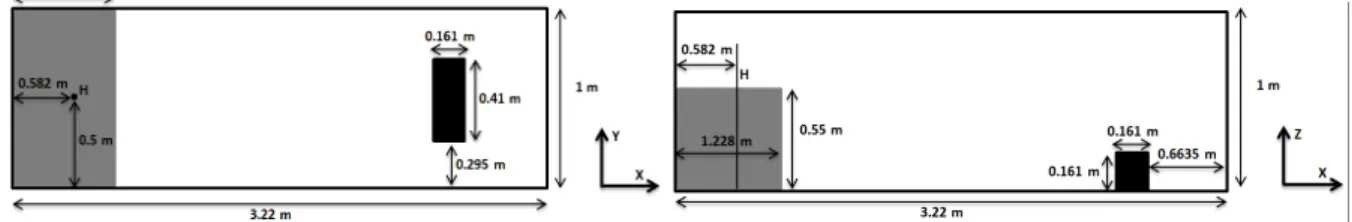
Computational setup
The geometry of the problem is described in Fig. 2. Free surface elevation was measured at point H and compared with experimental data (Kleefsman et al. (2005)). In this paper, the effect of time stepping algorithm, density filter and viscosity treatment has been
studied. The combinations of these parameters for all cases are shown in Table 1. The total time of simulation was 6 seconds. The focus of this study is on the accuracy of free surface simulation. Due to the computational limitations, the number of particles is only selected to be 52356.
Discussion of results
Based on the above description, twelve compiling options were studied. In fact, three time stepping algorithm, two density filters and two viscosity treatments were considered. The results of cases 3, 4, 6 and 8, shown in Table 1, cannot be presented. Due to the numerical errors which arise from the particles getting close to each other, simulations are stopped. Therefore, these options will be removed from the comparisons. In reality, by using these four options, the accurate results may not be achieved.
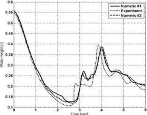
The time history of the free surface elevation at point H (shown in Fig. 2), for all cases, are illustrated in Fig. 3. It seems that the results from cases 5, 7, 9, 10 and 11 are not sufficiently accurate. However, it may be observed that, by using the results of cases 1, 2 and 12, accurate results for free surface elevation can be achieved. It is quite obvious that test case 12 gives more accurate results. To obtain more accurate results, the number of particles used in the simulation must be increased. For this purpose, the number of particles was increased to 94045. The obtained results are shown in Fig. 4. It is observed that the increase of the particle’s number leads to relative improvement of the results. Due to the computational restrictions, further increase of the number of particles could not be implemented. However, it may be concluded that by using more particles, better fitted results can be attained.
Figure 2. General description of the problem.
Table 1. Compiling options.
Time Stepping Method Density Filter Viscosity Treatment
Predictor-Corrector Verlet Symplectic None
Moving Least
Squares Artificial Laminar + SPS
Case 1 ∎ ∎ ∎
Case 2 ∎ ∎ ∎
Case 3 ∎ ∎ ∎
Case 4 ∎ ∎ ∎
Case 5 ∎ ∎ ∎
Case 6 ∎ ∎ ∎
Case 7 ∎ ∎ ∎
Case 8 ∎ ∎ ∎
Case 9 ∎ ∎ ∎
Case 10 ∎ ∎ ∎
Case 11 ∎ ∎ ∎
Case 1
Case 2
Case 5
Case 7
Case 9
Case 10
Case 11
Case 12
Figure 4. Numerical results versus experimental data by Kleefsman et al. (2005) for case 12 and computational cases of (Numeric #1 with 52356 particles) and (Numeric #2 with 94045 particles).
Conclusions
In this paper, a dam break problem was simulated by the smoothed particle hydrodynamics method. A variety of numerical features of 3D-SPH were probed to find a set of options which can be used to achieve more accurate numerical simulation. For this purpose, several numerical techniques such as time stepping algorithm, filter density and viscosity treatment were considered as compiling options. Twelve sets of mentioned schemes were also chosen and the elevation of free surface flow was captured. The predictor-corrector scheme, Verlet algorithm and Symplectic technique were considered as time stepping algorithms. The moving least square was also considered as a compiling option for the density filter. The viscosity treatment was also chosen based on the artificial viscosity and sub particle scale turbulence modeling. The numerical results were compared against the existing experimental data in the literature and it was found that the Symplectic algorithm in conjunction with density filter and SPS turbulence model can be used to achieve suitably accurate numerical results. It may be suggested that, in order to improve the numerical simulation, increasing the number of particles can be a good option. However, in the present study, due to the computational restrictions, the considered number of particle was only equal to 94045.
References
Benz, W., 1998, “Smooth particle hydrodynamics: a review”, In: J.R. Buchler, editor, The Numerical Modeling of Nonlinear Stellar Pulsations, pp. 269-288.
Colagrossi, A. and Landrini, M., 2003, “Numerical Simulation of Interfacial Flows by Smoothed Particle Hydrodynamics”, Journal of Computational Physics, Vol. 191, pp. 448-475.
Crespo, A., 2008, “Application of the smoothed particle hydrodynamics model SPHysics to free surface hydrodynamics”, Ph.D. thesis, University of De Vigo.
Dalrymple, R.A., Rogers, B.D., 2006, “Numerical modeling of water waves with the SPH Method”, Coastal Engineering, 53, pp. 141-147.
Del Pin, F., Idelsohn, S., Oñate, E. and Aubry, R., 2007, “The ALE/Lagrangian particle finite element method: a new approach to computation of free-surface flows and fluid-object interactions”, Computers & Fluids, Vol. 36(1), pp. 27-38.
Dilts, G.A., 1999, “Moving-Least Squares-Particle Hydrodynamics I. Consistency and Stability”, Int. J. Numer. Meth. Engineering, Vol. 44, pp. 1115-1155.
Gingold, RA., Monaghan, JJ., 1977, “Smoothed particle hydrodynamics— theory and application to non-spherical stars”, Mon. Not. R. Astron. Soc., Vol. 181, pp. 375-389.
Gomez-Gesteira, M. and Dalrymple, R.A., 2004, “Using a 3D SPH Method for Wave Impact on a Tall Structure”, J. Waterway, Port, Coastal and Ocean Engineering, Vol. 130(2), pp. 63-69.
Gotoh, H., Shibihara, T., and Hayashi, M., 2001, “Subparticle-scale model for the mps method lagrangian flow model for hydraulic engineering”, Computational Fluid Dynamics Journal, Vol. 9(4), pp. 339-347.
Kaceniauskas, A., 2008, “Development of Efficient Interface Sharpening Procedure for Viscous Incompressible Flows”, J. Informatica, Vol. 19(4), pp. 487-504.
Kleefsman, T., 2005, “Water Impact Loading on Offshore Structures”, PhD thesis, University of Groningen, The Netherlands.
Kleefsman, K.M.T., Fekken, G., Veldman, A.E.P., Iwanowski, B. and Buchner, B., 2005, “A volume of fluid based simulation method for wave impact problems”, J. Comp. Phys., Vol. 206, pp. 363-393.
Lee, E.S., Violeau, D., Benoit, M., Issa, R., Laurence, D., and Stansby, P., 2006, “Prediction of wave overtopping on coastal structures by using extended Boussinesq and SPH models”, In Proc. 30th International Conference on Coastal Engineering, pp. 4727-4740.
Lohner, R., Yang, C. and Onate, E., 2006, “On the simulation of flows with violent free surface, 2007 motion”, Comput. Methods Appl. Mech. Engrg., Vol. 195, pp. 5597-5620.
Lucy, LB., 1977, “A numerical approach to the testing of the fission hypothesis”, Astron. J., Vol. 82(12), pp. 1013-1024.
Monaghan, J.J., 1982, “Why particle methods work”, SIAM Journal on Scientific and Statistical Computing, Vol. 3(4), pp. 422-433.
Monaghan, J.J., 1992, “Smoothed Particle Hydrodynamics”, Annual Rev. Astron. Appl., Vol. 30, pp. 543-574.
Monaghan, J.J., 1994, “Simulating free surface flows with SPH”, Journal Computational Physics, Vol. 110, pp. 399-406.
Monaghan, J.J. and Kocharyan, A., 1995, “SPH simulation of multi-phase flow”, Computer Physics Communication, Vol. 87, pp. 225-235.
Monaghan, J.J. and Kos, A., 1999, “SolitaryWaves on a Cretan Beach”, J. Waterway, Port, Coastal and Ocean Engineering, Vol. 125, pp. 145-154.
Monaghan, J.J. and Kos, A., Scott Russells, 2000, “Wave Generator”, Physics of Fluids, Vol. 12, pp. 622-630.
Panizzo, A., 2004, “Physical and Numerical Modelling of Sub-aerial Landslide Generated Waves”, PhD thesis, Universita degli Studi diL'Aquila.
Panizzo, A. and Dalrymple, R.A., 2004, “SPH modelling of underwater landslide generated waves”, In Proc. 29th International Conference on Coastal Engineering, pp. 1147-1159.
Rogers, B.D., Dalrymple, R.A., 2004, “SPH modeling of breaking waves”, Proc. 29th Intl. Conference on Coastal Engineering. World Scientific Press, pp. 415-427.
Shao, S. and Gotoh, H., 2004, “Simulating coupled motion of progressive wave and floating curtain wall by SPH-LES model”, Coastal Engineering Journal, Vol. 46(2), pp. 171-202.