DYNAMIC APERIODIC NEURAL NETWORK FOR TIME SERIES PREDICTION

PORTUGUESE JOURNI'L OF MIWAGEMENT STUDIES, VOL. XJI, NO. 2, 2007

W

G

DYNAMIC APERIODIC NEURAL NETWORK FOR TIME SERIES

PREDICTION

Chiu-Che Tseng

Abstract

Department of Computer Science and Information Systems Texas A&M University-Commerce

There are many things that humans find easy to do that computers are currently unable to do. Tasks such as visual pattern manipulating objects by touch, and navigating in a complex world are easy for humans. Yet, despite decades of research, we have no viable algorithms for performing these and other cognitive functions on a computer. In this study, we used a bio-inspired neural network called a KA-set neural network to perform a time series predictive task. The results from our experiments showed that the predictive accuracy with this method was better in most markets than results obtained using a random walk method.

Keywords: Kset neural network, Time series, Prediction

INTRODUCTION

Neural Network technology was developed in an attempt to artificially reproduce the acquisition of knowledge and the organization skills of the human brain. It offers significant support in terms of organizing, classifying, and summarizing data, but with few assumptions and a high degree of predictive accuracy. Neural networks are less sensitive to error term assumptions; they can tolerate noise, chaotic components, and heavy tails better than most other methods. In this paper we apply a novel type of neural network, called KA sets. We selected the KA set neural network from traditional neural networks because results

PORTUGUESE JOURNAL OF MANAGEMENT STUDIES, VOL. X//, NO. 2, 2007

from experiments conducted by other researchers have shown that the KAlil model is a promising computational methodology for financial time series prediction [3], and it compares very well with alternative prediction methods.

A KA set is an abstract version of an already existing K set. Named after Aharon Katchalsky, an early pioneer of neurodynamics who tragically died in the early 70s, KA sets are strongly biologically motivated. KA models represent a family of models of increasing complexity that describe various aspects of. vertebrate brain functions. Similar to other neural network models, KA models consist of neurons and connections, thus their structure and behavior are more biologically plausible. The KA model family includes KAO, KAI, KAII, KAlil and KAIV.

Time series prediction takes an existing series of data. X(O), ... X(t-l),X(t), and forecasts the future values X(t+ l),X(t+2) .... etc. The goal is to model the history data in order to forecast future unknown data values accurately. Due to high noise level and the non-stationary nature of the data, financial forecasting is a challenging appjication in the domain of time series prediction. In this work we used the KAlil model to predict the one step direction of daily currency exchange rates.

RELATED WORKS

There are several studies using KA-set neural networks. Beliaev and Kozma [1] stored binary data in a Kill model and a Hopfield model. They then tried to retrieve the stored data by giving noisy input. The results of their study suggest that the K-model had greater potential for memory capacity than the Hopfield model.

Kozma and Beliaev [2] developed a methodology to use Kill for multi-step time series prediction and applied the method to the IJCNN CATS benchmark data.

Li and Kozma [3] applied a Kill dynamic neural network to the prediction of complex temporal sequences. In their paper, their Kill model gives a step-by-step prediction of the change in direction of a currency exchange rate.

PoRTUGUESE JOURNAL OF MANAGEMEtvr STUDIES, VDL. XI/, NO. 2, 2007

FOUNDATIONS OF THE KAlil NEURAL NETWORK

The architecture of artificial neural networks is inspired by the biological nervous system. It captures information from data by learning, and stores the information among its weights. Compared to other symbolic computational models, this computation model is especially good with regard to generalization and error tolerance. In a departure from traditional neural networks, the structure and behavior of the KA models are closer to the nervous system. Each KA set models some biological part of the nervous system, such as sensory pathways, cortical areas

etc. Another prominent difference from other generally known ~eural Networks is

that the activity of the K model is oscillatory, which is typically found within the chaotic regime.

The basic KA-unit, called KAO set, models a neuron population of about 10"' 4 neurons. It is described by a second order ordinary differential equation:

(a* b) d 2

P(t) +(a+ b) dP(t) + P(t)

=

d~

&

Here a and b are biologically determined time constants; a = 0.22, b =

0.72. P(t) denotes the activation of the nodes as function of time; F(t) is the summed activation from neighbor nodes ..

The KAO set has a weighted input and an asymptotic sigmoid function for the output. The sigmoid function Q(x) is given by the equation:

Q{x) = Q

* {

m

where Qm

=

the curve. This sigmoid function is modeled from experiments on biological neural activation.

FIGURE 1

Kl sets (a) excitatory Kl, (b) inhibitory Kl

b

PORTUGUESE JOURNAL OF MANAGEMENT STUDIES, VOL. XI/, NO. 2, 2007

P5(3)

P5(4)

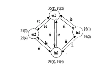
FIGURE 2

A KAII network

P6(3), P6(4)

P6(1)

P6(2)

The next step in the hierarchy is the KAII model. KAII is a double layer of excitatory or inhibitory units. In the simplest architecture there are 4 nodes: two excitatory and two inhibitory nodes;

Figure 2 shows the schema of the KAII set with two excitatory nodes (exl, ex2), and two inhibitory nodes (inl, in2). P5(i) and P6(i) are the activation levels and the derivatives of the activations of the excitatory and inhibitory nodes. They are called P5 and P6 for historical reasons.

In order to achieve a certain stability level on KAII, we conducted experiments to search for weight parameters, namely, ee, ii, ei, and ie, so that Kll can sustain oscillatory activation in impulse-response tests. Biological experiments have shown that when there is a single pulse of small random input perturbation, there are three types of Kll based on the activation trajectory of the excitatory node P5(1): positive attractor KAII, zero attractor KAII, and negative attractor KAII. The selection of weight parameters is based on satisfying these criteria. Three sets of KAII weight parameters are selected as in the following table:

TABLE I

KAII weights parameters

ei ie ee ii

Zero attractor KAII 1.0 2.0 1.8 0.8

Positive attractor KAII 1.6 1.5 1.6 2.0

Negative attractor KAII 1.9 0.2 1.6 1.0

PORTUGUESE JOURNAL OF MANAGEMENT STUDIES, VOL. XI/, NO. 2, 2007

The KAlil model is designed to be a dynamic computational model that simulates the sensory cortex. It can perform pattern recognition and classification. Based on the structure of the cortex, KAlil consists of three layers connected by feed forward/feedback connections. Each layer has multiple KAIJ sets, connected by lateral weights between corresponding P5(1) and P6(3) nodes. Based on the structure and dynamics of the sensory cortex, KAII sets in each layer should be zero attractor KAII, positive attractor KAII, and negative attractor KAII, respectively.

FIGURE 3

A sample KAlil network

Layer2

The schema of a KAlil set with three layers of KAII units with feed forward, feedback, and lateral connections is shown in Figure 3. It only shows two KAII sets in each layer. In order to get a homeostatic balanced state in the KAlil level, we list the activation equations for all 12 nodes in a single column in KAlil. The equation of P5(1) node in the first layer is:

P₁₅₀> =eel * f(P₁₅₍₃>)- iel * f(P₁₆₀) -iel *f(P₁₆(₃>) +Wee* f(P_{150 )}

+

*

In the above equation P₁₅₀>'P₁₅(

3>,P160>,P16(3> are the activations of the node P5(1), P5(3),P6(1) and P6(3) in layer 1; P₂₅m is the activation of P5(1) node in layer 2; eel and iel are the connections between KAII sets in layer 1. Wee is the

lateral connection between KAII sets in layerl; W P

25(l)Pl5(1> is the feedback connection from P ₂₅m node in layer 2 toP ₁₅m node in layer 1; f(x) is the asymmetric sigmoid function.

After plugging in the parameters in table I, we balance 12 nonlinear equations for each node. As a result, we get the parqmeters for all the lateral connections

PORTUGUESE JOURNAL OF MANAGEMENT STUDIES, VOL. X//, NO. 2, 2007

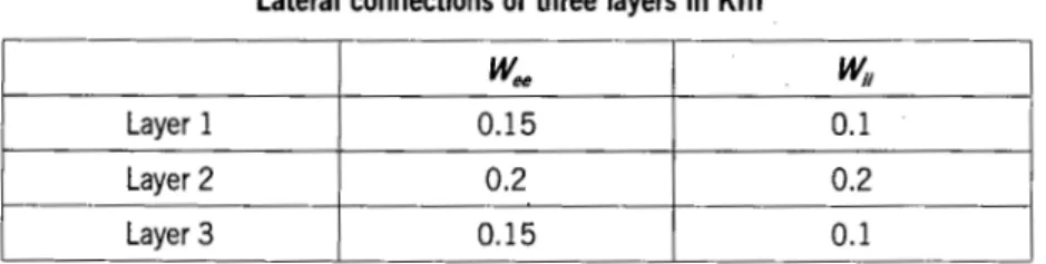
TABLE II

Lateral connections of three layers in Kill

w..,

Layer 1 0.15 0.1

Layer 2 0.2 0.2

Layer 3 0.15 0.1

Wee is the lateral connections between excitatory nodes; Wii is the connections between inhibitory nodes

TABLE Ill

Lateral connections of three layers in Kill

WP25(!)P!5(!) 0.05 Feedback Connection

WP25(!)P!6(!) 0.25 Feedback Connection WP36(l)P16(!) 0.05 Feedback Connection

WP!5(!)P25(!) 0.15 Feedforward Connection

W P35(!)P26(!) 0.2 Feedback Connection WP!5(!)P35(!) 0.6 Feedforward Connection

NEURAL NETWORK STRUCTURE AND LEARNING RULE

After the set up of KAlil to a homeostatic balanced state, its periodic dynamic can be sustained if the inputs are within a certain range. We constructed KAlil with different lateral nodes, varying from 2 to 60. This parameter decides the dimension of the input time series. For example, in a KAlil with 40 lateral nodes, the inputs for each excitatory node are X(t-40), X(t-39) ... X(t-1). If the previous 40-day currency exchange rates are entered into the system, our model will predict the change in direction of the next day's rate.

The learning rule in KAlil is associative Hebbian learning. Since the system is always in a dynamic state, there is no single converged value. The activation standard deviation (cri) of each node in a certain duration T is used.

~Wij

=

PORTUGUESE JOURNAL OF MANAGEMENT STUDIES, VOL. XI/, NO. 2, 2007

a.=_!_

f

2

(5)

I T 0 I T£... l

t=l

In the discrete version we use

cr. =[ 1 _I IT~- _{I= 1} T (P35.(t) -1/T _I ~ _{\ = 1} TP35.(t))2] _I 1'2

where T = 200 ms, P35i(t) is the activation of excitatory node at instant tin layer 3; cr is defined as the mean of the cri.

cr= 1

I

1=1

(6)

where L is the number of lateral nodes.

MYOPIC STRATEGY

In the domain of time series prediction, in order to predict the next output data, we need to determine what is the right input size to use. For example, should we use the prior 30 days' index data as input and predict the data on the 31st day or should we use a different input size? In this study, we applied a myopic strategy to find the right input size to use for predicting the following day's output. The strategy starts with 2 inputs and constructs the KAII network accordingly. It will then increase the input size and so on. The strategy will stop when the accuracy rate produced by the network has reached a preset threshold. The result network will be selected for the particular data set.

This approach saves a considerable amount of computational time over the trial and error approach for selecting the right input size to use for the data set.

EXPERIMENTAL SETUP

PORTUGUESE JOURNAL OF MANAGEMENT STUDIES, VOL. XI/, NO. 2, 2007

We did not fix the L value, i.e. the learning rate, at 40 nodes. Instead, we used a myopic strategy to try all possible input sizes, varying L value from 2 to 60 nodes. The best L value was then determined on the basis of the results.

DATA NORMALIZATION

The data used were the stock index data of eight different countries from the period of 1986 to 2004. We normalized the data so that they were in the range of [-1,1]. This was done by taking the difference between two corresponding data values and dividing them with the maximum of all difference values present. We had more than four thousand data points of the daily closing bids of each country's stock index data. Due to the nature of the KAlil, the same input needs to be repeated for a certain duration, then followed by a period of relaxation (zero input). This is a biologically inspired process to mimic the activity of a sniff and other sensory activities. We chose both the learning and relaxation durations to be 25minutes in this work.

LEARNING PHASE

Prior to putting learning data into KAlil, each input was labeled as UP/SAME/ DOWN according to the next data. The Hebbian learning process happens in the lateral connections among the excitatory nodes in the third layer. As explained in the previous section, the learning phase lasted 25minutes. In our experiment, the first 5 minutes' response activations were skipped because initial activations are considered unstable when the signal is first perceived by the system. Thus, only the following 20minutes' activations of e~citatory nodes P35(1) in layer 3 were collected for learning purposes. We plugged these data into the Hebbian learning equation. The lateral connections were adjusted accordingly. We called this process a cycle. The learning cycle was repeated for two thirds of the data. Observing the weight change indicates that some weights increased, while some decreased during learning.

VALIDATION PHASE

PORTUGUESE JOURNAL OF MANAGEMEIVT STUDIES, VOL. XI/, NO. 2, 2007

references to classify patterns in the testing phase. From the point of view of aperiodic dynamics, the values of the spatially distributed oscillation intensities encode the input data. When a given input is applied, the high dimensional dynamics collapse to a lower dimensional subspace. In other words, these oscillatory patterns generate the clusters for different categories.

TESTING PHASE

During the testing phase, the filtered standard deviations were recorded for each group of testing data. These were defined as the activation points for the testing data. Then, the distances from all references to the activation point were calculated. The classification algorithm selected theN references with the smallest distances. Our classification algorithm required that the difference between the numbers of references belonging to each pattern be greater than others in order to claim a "winner". The "winner" pattern decides which pattern the testing data belongs to. For example, for each case there are 9 nearest neighbors. In Case 1, 6 references belong to pattern UP and 3 references belong to pattern DOWN. The system would classify the UP category as the "winner" for this testing point.

In Case 2, if 5 references are pattern UP, and 4 references are pattern DOWN, the system classifies the testing data "winner" as the UP category. The size of the neighborhood N which decides the "winner" is acquired from the experiment in the testing phase. We used the first one third of testing data to try some N values. We checked the classification performance for every N configuration. The N configurations with the best performance were selected for the following two-thirds of the testing data. Once N was decided, they would remain constant for all of the following testing data. Therefore, only two-thirds of the testing data were counted as performance evaluation in each test run.

EXPERIMENTAL RESULTS

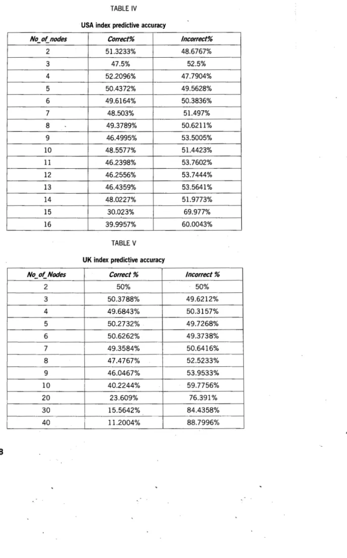
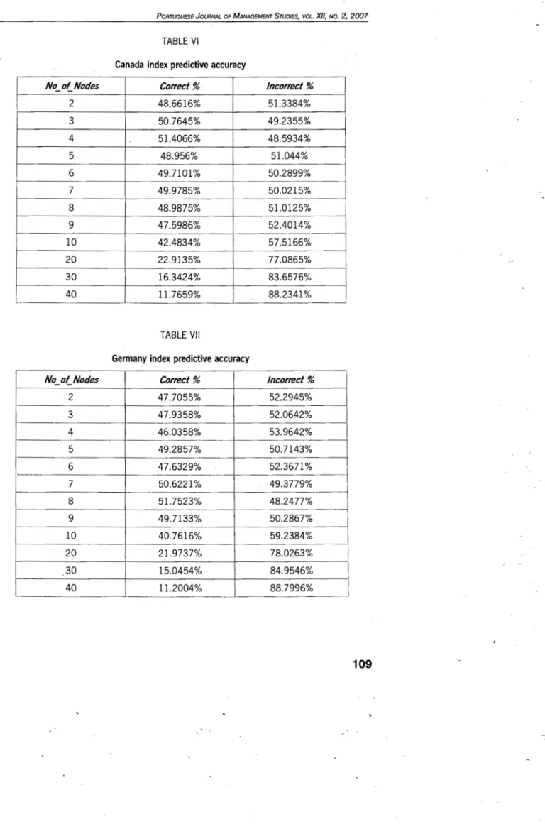
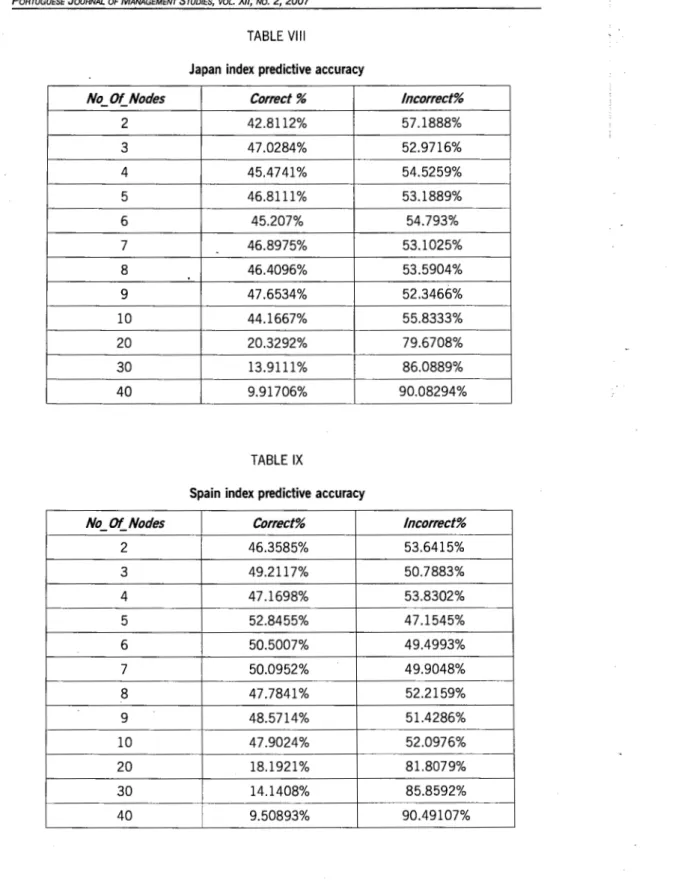
We ran through all eight markets' stock index data using out myopic KAII neural network and we got different results from different markets. Most of the predictive accuracy rates were more than 50%, only Japan's market did not attain more than 50%.

PORTUGUESE JOURNAL OF MANAGEMENT STUDIES, VOL. X//, NO. 2, 2007

TABLE IV

USA index predictive accuracy

No_ot_nodes Correct% Incorrect%

2 51.3233% 48.6767%

3 47.5% 52.5%

4 52.2096% 47.7904%

5 50.4372% 49.5628%

6 49.6164% 50.3836%

7 48.503% 51.497%

8 49.3789% 50.6211%

9 46.4995% 53.5005%

10 48.5577% 51.4423%

11 46.2398% 53.7602%

12 46.2556% 53.7444%

13 46.4359% 53.5641%

14 48.0227% 51.9773%

15 30.023% 69.977%

16 39.9957% 60.0043%

TABLE V

UK index predic!ive accuracy

No_ of_ Nodes Correct% Incorrect%

2 50% 50%

3 50.3788% 49.6212%

4 49.6843% 50.3157%

5 50.2732% 49.7268%

6 50.6262% 49.3738%

7 49.3584% 50.6416%

8 47.4767% 52.5233%

9 46.0467% 53.9533%

10 40.2244% 59.7756%

20 23.609% 76.391%

30 15.5642% 84.4358%

40 11.2004% 88.7996%

PORTUGUESE JoURNAL OF MANAGEMENT STUDIES, VOL. XI/, NO. 2, 2007

TABLE VI

Canada index predictive accuracy

No_ of_ Nodes Correct% Incorrect%

2 48.6616% 51.3384%

3 50.7645% 49.2355%

4 51.4066% 48.5934%

5 48.956% 51.044%

6 49.7101% 50.2899%

7 49.9785% 50.0215%

8 48.9875% 51.0125%

9 47.5986% 52.4014%

10 42.4834% 57.5166%

20 22.9135% 77.0865%

30 16.3424% 83.6576%

40 11.7659% 88.2341%

TABLE VII

Germany index predictive accuracy

No_ of_ Nodes Correct% Incorrect%

2 47.7055% 52.2945%

3 47.9358% 52.0642%

4 46.0358% 53.9642%

5 49.2857% 50.7143%

6 47.6329% 52.3671%

7 50.6221% 49.3779%

8 51.7523% 48.2477%

9 49.7133% 50.2867%

10 40.7616% 59.2384%

20 21.9737% 78.0263%

30 15.0454% 84.9546%

PORTUGUESE JoURNAL OF MANAGEMENT STUDIES, VOL. X//, NO. 2, 2007

TABLE VIII

Japan index predictive accuracy

No_ Of_ Nodes Correct% Incorrect%

2 42.8112% 57.1888%

3 47.0284% 52.9716%

4 45.4741% 54.5259%

5 46.8111% 53.1889%

6 45.207% 54.793%

7 46.8975% 53.1025%

8 46.4096% 53.5904%

9 47.6534% 52.3466%

10 44.1667% 55.8333%

20 20.3292% 79.6708%

30 13.9111% 86.0889%

40 9.91706% 90.08294%

TABLE IX

Spain index predictive accuracy

No_ Of_ Nodes Correct% Incorrect%

2 46.3585% 53.6415%

3 49.2117% 50.7883%

4 47.1698% 53.8302%

5 52.8455% 47.1545%

6 50.5007% 49.4993%

7 50.0952% 49.9048%

8 47.7841% 52.2159%

9 48.5714% 51.4286%

10 47.9024% 52.0976%

20 18.1921% 81.8079%

30 14.1408% 85.8592%

PORTUGUESE JOURNAL OF MANAGEMENT STUDIES, VOL. XI/, NO. 2, 2007

TABLE X

Taiwan index predictive accuracy

No_ of_ Nodes Correct% Incorrect%

2 50.2342% 49.7658%

3 48.7828% 51.2172%

4 48.0408% 51.9592%

5 48.6486% 51.3514%

6 49.4069% 50.5931%

7 47.3379% 52.6621%

8 47.2222% 52.7778%

9 47.8128% 52.1872%

10 37.8175% 62.1825%

20 19.819% 80.181%

30 13.6426% 86.3574%

40 10.6429% 89.3571%

TABLE XI

Singapore index predictive accuracy

No_of_Nodes Correct% Incorrect%

2 49.4715% 50.5285%

3 48.1293% 51.8707%

4 51.8362% 48.1638%

5 48.693% 51.307%

6 50.0534% 49.9466%

7 53.3078% 46.6922%

8 52.921% 47.079%

9 48.6014% 51.3986%

10 41.2635% 58.7365%

20 20.8025% 79.1975%

30 14.7407% 85.2593%

PORTUGUESE JOURNAL OF MANAGEMENT STUDIES, VOL. XI/, NO. 2, 2007

FIGURE 4

The best predictive accuracy from KAlil neural network in different markets

Gl 54

~53

1: 52

8 51 ; 50

~ 49

·;. 48

~ 47

5 46

8 45

c(44

CONCLUSION

vr-;t

Markets

Our initial research on using a neurodynamic Kill network on different stock markets' index data prediction produced good results. We plan to further our research by applying it to other domains, including health and human activity modeling.

References

Atiya, A., and Parlos, A, (1995), "Identification of nonlinear dynamics using a general spatia-temporal network,", Math. Compute Modeling J. Vol. 21, no. 1, pp. 55-71, Jan.

Bassi, D., (1995) Stock price predictions by current by recurrent mu/tiplayer neural network

archi-tectures in the Capital markets Conf., A. Reference Ed. London, U.K., October 1995, London

Business School, pp. 331-340.

Beliaev, Igor, Kozma, Robert (2007) "Time Series Prediction Using chaotic Neural Networks: Case Study of ljcnn Cats Benchmark Test", Department of Mathematical Sciences, University of Memphis, Memphis, TN.

Beliaev, Igor, Kozma, Robert (2006), "Studies on the Memory Capacity and Robustness of Chaotic

Dynamic Neural Networks", International Joint Conference on Neural Networks, Vancouver,

BC, Canada, July 16-21.

Carney, J.G., Cunningham (1996), "Neural networks and currency exchange rate prediction", Fore-sight Business Journal, http://www.maths.tcd.ie/pub/fbj/index.html.

Chang, H.Z., Freeman, W.J. and Burke, B.C. (1998), "Optimization of Olfactory Model in Software to Give 1/f Spectra Reveals Numerical Instabilities in Solutions Governed by Aperiodic (cha-otic) Attractors", Neural networks, 11, 449 -466.

Freeman, W.J. (1975) Mass Action in the Nervous System, Academic Press, N.Y.

Gardner, E., Derrida B., (1988), "Optimal storage properties of neural network models", Journal of

PoRTUGUESE JouRNAL OF MANA(JEMENT STUDIES, voL. XII, NO. 2, 2007

Giles, C.L., Lawrence, S. and Tsoi A.C. (2001), Noisy time series prediction using a recurrent neural network and grammatical inference, Machine earning, 44 (1-2), pp. 161-183. Hopfield, J.J. ,(1982), " Neural Networks and Physical Systems with Emergent Collective

Computa-tional Abilities", Proc. Natl. Acad. Sci., USA, Volume 79, pp. 2554-Z558.

Kozma, R., Freeman W.J., and Erdi, P., (2003), The Kiv Model- Nonlinear spatia - temporal

dynamics of the primordial vertebrate forebrain; Neurocomputing, 2003 in press.

Li Haizhon, Kozma, Robert (1982), "A dynamic Neural Method for time Series Prediction Using the Kill Model" Division of Computer Science, University of Memphis, Memphis, TN.

McEiiece, R.J., Posner, E.C. Posner, Rodemich, E.R. and Venkatesh, S.S., (1987) "The capacity of the Hopfield associative memory", IEEE Trans. Inform. Theory, Vol. 33, pp. 461, July 1987.

Moody, J. and Wu L. (1996), Optimization of trading systems and portfolios, in Proc. Neural

Networks Capital Markets Cont. Pasadena, CA.

Mueller, B., Reinhardt (1990), "Neural Networks: An Introduction", Springer.

Muthu, S., Kozma, R., Freeman W.J. ( 2004), "Applying KIV dynamic neural network model for real time navigation by mobile robot Aibo", lEE/INNS 2004 Int. Joint Conference on Neural net-works IJCNN'04, July 25-29, 2004 Budapest, Hungary.

Toomarian, N. and Barthen, J. (1991), "Adjoint -functions and temporal learning algorithm in neural networks", Advances in neural information Processing Systems, 3, pp. 113- 120.

Resumo

Ha muitas coisas que o Homem tern facilidade em fazer e que os computadores actuais nao tern ainda essa capacidade. Par exemplo, manipular objectos atraves do tacto e navega<;ao num mundo com-plexo sao tarefas faceis para os seres humanos. Apesar da investiga<;ao realizada ao Iongo de varias decadas, nao ha algoritmos suficientemer:~te validos para realizar estas e outras fun<;6es cognitivas no computador.

- Neste estudo utiliza-se urn sistema "bio - inspirado" numa rede neuronal designada par "KA-set neural network" para efectuar previs6es de series temporais. Os resultados do estudo demonstram que a precisao de previsao deste metoda foi melhor na maioria dos mercados do que os resultados obtidos par urn metoda aleat6rio.