Abstract
For realistic applications, design and control engineers have lim-ited modelling options in dealing with some vibration problems that hold many nonlinearity such as non-uniform geometry, varia-ble velocity loadings, indefinite damping cases, etc. For these reasons numerous time consuming experimental studies at high costs must be done for determining the actual behaviour such nonlinear systems. However, using advantages of multiple compu-tational methods like Finite Element Method (FEM) together with an Artificial Intelligence (ANN), many complicated engineering problems can be handled and solved to some extent. This study, proposes a new collective method to deal with the nonlinear vibra-tions of the barrels in order to fulfil accurate shooting expectan-cy. Using known analytical methods, in practical, to determine dynamic behaviour of the barrel beam is not possible for all condi-tions of firing that include numerous varieties of ammunition for different purposes, and each projectile of different ammunition has different mass and exit velocity. In order to cover all cases this study proposes a new method that combines a precise FEM with ANN, and can be used for determining the exact dynamic behav-iour of a barrel for some cases and then for precisely predicting the behaviour for all other possible cases of firing. In this study, the whole nonlinear behaviour of an antiaircraft barrel were ob-tained with 3.5% accuracy errors by ANN trained by FEM using calculated analysis results of ammunitions for a particular range. The proposed FEM-ANN combined method can be very useful for design and control engineers in design and control of barrels in order to compensate the effect of nonlinear vibrations of a barrel for achieving a higher shooting accuracy; and can reduce high-cost experimental works.
Keywords
Nonlinear vibration modelling, Vibration of continuous systems, Artificial neural networks, Gun barrels, Finite element method
Tip Deflection Determination of a Barrel for the Effect
of an Accelerating Projectile Before Firing Using Finite
Element and Artificial Neural Network Combined Algorithm
Mehmet Akif Koç a
İsmail Esen b
Yusuf Çay c
a Department of Mechanical Engineering,
Sakarya University, Sakarya, Turkey. [email protected]
b Department of Mechanical Engineering,
Karabük University, Karabük, Turkey [email protected]
c Department of Mechanical Engineering,
Sakarya University, Sakarya, Turkey. [email protected]
http://dx.doi.org/10.1590/1679-78252718
1 INTRODUCTION
The non-linear dynamic behaviour of a structure due to the effect of an accelerating mass is still a research interest with the applications of it in the new fields such as defence and transportation engineering. The effects of moving loads on the dynamics of the structures have been widely stud-ied in literature, for example, (Dehestani et al., 2009; Lee, 1996; Michaltsos, 2002; Niaz and Nikkhoo, 2015; Omolofe and Oni, 2015; Wang, 2009) have investigated the subject. For the appli-cation to the bridge engineering (Michaltsos et al., 1996) have studied the effect of accelerating ve-hicles on the bridge beams, considering highway bridges and high speed rail road construction. Some more accurate tools of engineering calculations of the dynamic interaction using FEM have been proposed by(Esen, 2011, 2015, 2013; Kahya, 2012) . Using analytical methods for simple cases neglecting damping effects and assuming uniform beam cross sections (Esmailzadeh and Jalili, 2003; Liu et al., 2015; Wyss et al., 2011) have studied the subject in terms of vehicle structure interaction problems. Using a two-axle half car model, (Lou, 2005) has studied the wheel - rail interaction and dynamics of a railway bridge. For both simple and realistic models of moving vehicles can be found in(Azimi et al., 2013; Lou and Au, 2013; Yang et al., 2013).
The moving mass problem is also vital in defence field, but the studies in this field are rarely available in literature due to the confidentiality. Using a precise FEM model(Esen and Koç, 2015a) have presented the interaction of an accelerating projectile and a barrel of a cannon. Effect of stepped barrels on the stability and the dynamics of barrels have been investigated by (Balla, 2011; Tawfik, 2008). In order to understand interaction between projectile and barrel, (Alexander, 2007) has prepared an ABAQUS explicit dynamic finite element model, and then compared analysis re-sults to the test data 155 mm cannon. M. Stiavnicky and P. Lisy, 2013 have investigated numerical simulation to determine influence of the barrel fixing on barrel vibration when bullet exits barrel. Another aspect of reducing the vibrations is the usage of dynamic vibration absorbers, and (Esen and Koç, 2015b; Kathe, 1997; Littlefield et al., 2002) have studied the vibration reduction of bar-rels.
ANN also known as ‘parallel distributed processing’ is a powerful artificial intelligence for solv-ing complicated engineersolv-ing problems. This method can be applied to predict the desired output parameters when the database of the problem represents all relationships. ANN have been used in different engineering applications such as mechanical vibrations (Koide et al., 2014; Lagaros and Papadrakakis, 2012; Liu et al., 2015; Martínez-Martínez et al., 2015; Perez-Ramirez et al., 2016) rail rolling processing (Altınkaya et al., 2014), creep modelling (Düğenci et al., 2015), steel projectile penetration depth (Hosseini and Dalvand, 2014) and internal combustion engines to estimate some important parameters of fuels on emissions (Cay, 2013; Czarnigowski, 2010). The uses of ANN in the field of defence systems have recently begun to increase. ANN models have played an im-portant role in the development of military automatic target recognition (ATR) (Rogers et al., 1995).
example, for a tank system, there are various classes of ammunition for different purposes, and each projectile of different ammunition has different mass and exit velocity. In order to cover all cases, this study proposes a new method that combines a precise FEM with an artificial intelligence tech-nique ANN, and can be used for determining the dynamic behaviour of the barrel for some cases and then for precisely predicting the behaviour for all other possible cases of firing. The proposed FEM-ANN combined method can be very useful for control engineers in design of fire control algo-rithm of weapon in order to compensate the effect of nonlinear vibration of a barrel for achieving a higher shooting accuracy. There should be many compensation sub systems in a weapon system in order to satisfy the shooting accuracy that is the most important property in such systems. Howev-er, in order to design a proper compensation system, engineers need very large data about the dy-namic behaviour of the barrels. The needed data can be created by means of experimental studies, but experimental studies are generally time-consuming and expensive. As an alternative to the ex-perimental studies, one of the economic ways of creating accurate data is the modelling using the prediction power of artificial intelligence techniques. In this study, the mass and exit velocity of a projectile are used as input, while the tip deflection as output, and the predictions of the deflections have been achieved with an acceptable accuracy. Where, the R2 is 0.99 for training and testing; the MSE for training is 8.25x10⁻⁴, for testing is 0.03767; the MEP, for training is 0.5%, for test is 0.1%.
Without omitting all the nonlinearities including damping, this method can also easily be adapted to other problems of the structural dynamics such as vehicle bridge interaction, wheel/rail interaction, high-speed precise machining, and flexible run-ways of robotic systems, etc. Being ca-pable of predicting the nonlinear behaviour for many cases, this technique can reduce research and development costs by reducing costly and time-consuming experimental studies.
2 MATHEMATICAL MODELLING
In the formulation, the following assumptions will be adopted (Fig. 1) The mass inertia is considered.
The mass is always in contact with the beam.
The beam is thin and small displacements in the beam occurred according to thin beam theo-ry.
The beam is of variable thickness and the material properties are constant trough length of the beam.
The trajectory of the mass is defined by time-dependent xp(t)
Based on the above assumptions, the motion equation of the barrel beam due to the effect of the projectile located at the time-dependent point xpwithin the barrel beam, is provided by Eq. (1)
(L. Fryba, 1999):
4 2
4 2
2
2
( , ) ( , ) ( , )
( ) ( ) ( , ),
d ( , )
( , ) ( (t)) ( (t))
d
z z z
z p
p p p p
w x t w x t w x t
EI x A x F x t
t
x t
w x t
F x t m g x x m x x
t
r s
d d
¶ ¶ 
+ + =
¶ 
æ ö÷
ç ÷
ç
= - - ç ÷
-÷÷
çè ø
The left hand side of Eq. (1) represents the resisting internal stiffness, inertia and damping forc-es due to the external forcforc-es on the right side. Where, ρ is the density, A(x) is the none-uniform
cross-sectional area, σis the equivalent viscous damping coefficient, E is the Young’s modulus of
elasticity; I(x)is the area moment of inertia, while x represents the central coordinate of the barrel
system; t represents time; w(x, t) is the vertical displacement of the barrel; mp is the mass of the
projectile; m g xp d( -xp(t)) is the force applied to the unit length of the barrel by the projectile (as a moving mass); while g anddrepresent gravitational acceleration and the Dirac delta function,
respectively; and d2w(x
p, t)/dt2 represents the acceleration of the barrel at the contact point of
lumped projectile mass. For inclined positions of the barrel beam one can refer to the study by Esen and Koç, 2015b.
The initial and boundary conditions of the barrel beam are:
¶ =
= = =
¶ ( , 0) ( , 0) w x t 0 w x t
t (2a)
¶ =
= = =
¶ = = ¶ = =
¶ 
2 3
2 3
( 0, )
( 0, ) 0, 0
( , ) ( , )
0, 0 w x t
w x t
x
w x L t w x L t
x x
(2b)
In order to determine time dependent displacements of the barrel tip, which is very important for shooting accuracy of the weapon, a rough analytical solution of the motion Eq. (1) can be ob-tained through some simplifications by ignoring the effects of inertia and damping, and accepting that the cross-section area is uniform and the projectile moves with a constant velocity. For simpli-fied cases, that omits geometric and dynamic nonlinearities, such moving load problems have been extensively studied in the literature by numerous researchers. From this perspective, the proposed FEM-ANN combined method can be very useful for design and control engineers if they pay atten-tion to the requirements of modelling as described below.
The model of the barrel with an accelerating projectile is shown in Figure 1. The interaction of the barrel and the projectile are determined in both vertical and horizontal directions.
z
r, A(x), L, E, I(x)
m
,v (t)
m
x
a (t)
l
q
p
v
u
1
1 1
2
q
p,
m v
2
u2
wz (L,t)
x
wz (x,t)
s Beam elementth
While the barrel is vibrating, the transverse and longitudinal interaction forces between the barrel and the projectile that is accelerating trough the deflected barrel geometry can be determined by using the following equation (Cifuentes, 1989; L. Fryba, 1999):
d
d
=
é¶ ¶ ù
ê + ú
ê ¶ ¶ ú
ê ¶ ú
ê ú
= - ê æ ö ú
-¶ ç ÷÷ 
ê+ çç ÷÷ + ú
ê ¶ çç ÷÷ ¶ ú
è ø ê ú ë û = -= + + = + 2 2 2 2 2 2 2 2 2 2 2 2
0 0 0 2
d ( , ) ( , ) 2 d ( , ) [ ] ( ) d d ( , ) ( , ) d d
d ( , )
( , ) ( )
d
d d
; ;
2 d d
p
p
z z
z p p p
p p
z z
x x
x p
x p p
p p
m
p m
x
w x t w x t
x t t
t
f x t m g m x x
x x
w x t w x t
t x
x t
w x t
f x t m x x
t
x x
a t
x x v t v a t
t t =am
(3)
In above equation fz(x,t) and fx(x,t) respectively, are transverse and horizontal contact forces
between the barrel and the projectile accelerating at point xp on the axis, while t represents time,
while (x-xp) and g are the Dirac-delta function and the gravitational acceleration, respectively.
The parameters x0 and v0 are the initial position and initial speed of the projectile at time t=0,
re-spectively. On the other hand, am is the average acceleration of the projectile within the barrel.
Under the effect of the accelerating projectile, the equivalent nodal forces of the barrel element (Figure 2 a and b) and the relationships between the shape functions and the transverse and longi-tudinal deflection functions and the nodal displacements of the sth element at position x
m(t) at time
t are as follows:(Clough R.W; Penzien J., 2003):
y y
y y
y y q y y q
= = ¢ ¢¢ ¢ = + + + + + + = = + = + + +
2
0 0
1 1 4 2
2 1 3 1 5 2 6 2
( 1, 4)
( 2 ( ) ( ) ) ( 2, 3, 5, 6) ( , )
( , )
i i p x
i i p z z m z m m z
x z
f m w i
f m w w v a t w v a t a w g i
w x t u u
w x t v v
(4)
(
)
(
)
y x y x
y x x y x x
y x x x y x x
x = - = = - + = -= - + = - + = 1 4
2 3 2 3
2 5
2 3 2 3
3 6
1 ( ) ( )
1 3 ( ) 2 ( ) 3 ( ) 2 ( )
( ) 2 ( ) ( ) ( ) ( )
( ) ( ) m
t t
t t t t
t t t l t t l
x t t
l
(5)
In these expressions, “ ′ ” and “ . ” represent the spatial and time derivatives of the displace-ment function, respectively. In addition, wz=wz(x,t) and wx=wx(x,t) represent the vertical
displace-ment (z) and Longitudinal (x) on the coordinate plane of the barrel at coordinate x and time t. The
are represent axial displacement, vertical displacement and slope, respectively.
i(i=1-6) are theshape functions of the beam element (Clough R.W; Penzien J., 2003) . The length of the element is
l. and xm(t) is the variable distance between the accelerating projectile and the left end of the sth
element at time t as shown in Figure 2b.
Figure 2: Modelling of the barrel and projectile interaction using FEM a-) FEM discretion of the barrel system b-) Beam element s over which the projectile mp passes at time t.
The property matrices of a beam element in Figure 2, having transverse and longitudinal nodal forces and displacements, can be derived from the procedure of the principle of virtual work and the relation of the kinetic and internal potential energies of the element.
In the case of interaction with a projectile, any stiffness coefficient associated with beam flexure and axial displacements for the element on which the projectile locates is as follows:
(
)
(
)
2 0 0 0( ) ( ) ( ) ( ) , ( ) , , 2, 3, 5, 6
( ) ( ) , , 1, 4
l
ij i j i j m i j m
l
ij i j
k EI x x x dx v t a v t v a t i j
k EA x x dx i j
y y y y y y
y y ¢¢ ¢¢ ¢¢ ¢ = + + = + = ¢ ¢ = - =
ò
ò
(6)In the same manner, for the relation between nodal accelerations and resisting inertial forces, the elemental balance equation can be obtained. Including the effect of the projectile, any mass coefficient associated with beam flexural and axial accelerations are as follows:
y y y y y y y y y y
y y y y y y
é ù é ù
= + êë ú êû ë úû
=
é ù é ù
= + êë ú êû ë úû
=
ò
ò
2 3 5 6 2 3 5 6
0
1 4 1 4
0
( ) ( ) ( ) 0 0 0 0
, (2, 3, 5, 6)
( ) ( ) ( ) 0 0 0 0 0 0 0 0
, (1, 4)
l
T
ij i j p
l
T
ij i j p
m m x x x dx m i j m m x x x dx m
i j
(7)
The damping in the system can be any type; and for structural systems, hysteric and structural damping may be applied. However, considering practical usage in engineering any type of damping can be modelled as viscous damping using equivalent damping approximations. In this study, the
L
n+1
1
l
z
x (t)p
1 2
nodes am v (t) m mp Barrel n s th l
s element m
m x m(t)
s1 s1 f ,u
s-1 s+1
s2 f ,us2
f ,us3 s3 f ,us6 s6
f ,us5 s5
f ,us4 s4
amv (t) p
in which the damping matrix is proportional to the combination of the mass and stiffness matrices; and including the effect of accelerating projectile, the coefficients of time dependent damping matrix can be formed as follows:
(
)
(
)
a k y y y y y y y y
w w z w x w z w z w
a k
w w w w
é ù é ù
é ù= é ù+ é ù+ ¢ ¢ ¢ ¢
ê ú ê ú ê ú ê ú ê ú
ë û ë û ë û ë û ë û
-
-= =
-
-, , , 2 3 5 6 2 3 5 6
2 2 2 2
2 ( ) 0 0 0 0
2 2
,
T i j i j i j p
i j i j j i j j i i
j i j i
c m k m v t
(8)
where ziand zj are the damping ratios of the structural system for any corresponding natural fre-quencies ωiand ωj. The instantaneous equation of motion for the entire system is can be expressed
as:
{ }
{ }
{ } { }
é ù +é ù +é ù =
ê ú ê ú ê ú
ë ûM U t( ) ë ûC U t( ) ë ûK U t( ) F t( ) (9)
where [M], [C ] and [K ] are, respectively, the instantaneous overall mass, damping and stiffness
matrices, while
{ ( )}
U t
,{ ( )}
U t
and { ( )}U t are, respectively, the acceleration, velocity, and dis-placement vectors. Besides,{ }
F t( ) is the overall external force vector of the system at time t. Forthe obtaining the matrices of [M], [K], and [C], one can determine the elemental property matrices;
and then can assemble them properly using the conventional FEM approach. In case of an acceler-ating projectile the time dependent elemental matrices of the beam element s are determined using
the coefficients given Eqs. (6, 7 and 8). For calculation of time dependent property matrices, the instantaneous values of xm(t) and s are:
( ) ( ) ( 1)
m p
x t =x t - -s l (10a)
(integer part of ( ) / )p 1, (1 )
s= x t L + s= -n (10b)
Embedding the other inertia, centripetal and Coriolis forces in the left side of the system equa-tion, only the vertical gravitational and longitudinal acceleration force components of moving pro-jectile should be applied as external forces; thus, the instantaneous overall force vector becomes as follows:
( )
0 ... 1 2 3 4 5 6 ... 0 ,
( 2, 3, 5, 6), ( 1,4)
T
s s s s s s
s i p i s i p m i
F t f f f f f f
f m g
i f m a
i
(11)
3 ARTIFICIAL NEURAL NETWORK MODELLING TO PREDICT THE AMOUNT OF TIP DIS-PLACEMENT
the human brain. Thanks to the discovery of new information, learning refers to the process of improvement in behaviour in living beings. On the other hand, Machine learning refers to a situa-tion where all of these operasitua-tions are conducted by a computer. To be able to learn, computers require a dataset on the event in question, thus learning through artificial neural networks requires a training set. Examples in the training set are based on previous experience with the problem in question. Learning is achieved by introducing these examples to the neural network in an order. Artificial neural networks are computer systems that are able to learn and to react to stimuli in the environment by making use of previous examples implemented by humans. At a most basic level, the task of an artificial neural network is to produce a set of outputs that correspond to given in-puts. For the artificial neural network to be able to do that, the network needs to be trained by existing examples of events representing the engineering problem in question, and eventually needs to acquire the ability to generalize.
The most important parameter that affects the shooting accuracy of a weapon system is the vertical movement of the muzzle, which happens during shooting, also known as a muzzle displace-ment. These movements cause the barrel axis to displace, and have an adverse effect on the shoot-ing accuracy of the weapon system. Considershoot-ing the long ranges of contemporary weapon systems, small muzzle displacements can result in large deviations from the target. Muzzle displacements are affected by two basic parameters. The first of these parameters is the velocity of the projectile as it departs from the muzzle, and the second is the force of gravity perpendicular to the muzzle axis, due to the mass of the projectile. Contemporary firearms, in particular, are designed to have larger projectile masses and higher muzzle velocities in order to be more effective against rapidly moving and manoeuvring targets. However, larger projectile masses and higher muzzle velocities have generated serious problems on the target accuracies of weapons.
To deal with this problem, a number of active and passive control systems have been designed. For example, some studies (Esen and Koç, 2015a; Littlefield et al., 2002) report that when a mass-spring system is added to the muzzle, it is able to decrease muzzle displacement by around 50%. However, this technique was not able to eliminate muzzle displacement, which could be due to a number of reasons. One reason is that the projectile forces the barrel to change its frequency con-tinuously until it departs the muzzle, making it difficult to design an appropriate absorber. In ad-dition, even if an absorber were to be designed that matches the forcing frequency of the projectile, the natural frequencies of the whole system change when the absorber is mounted on the barrel. All of these factors limit the use of passive vibration absorbers on gun barrels. Active control sys-tems have also been designed to prevent muzzles from dipping. However, these syssys-tems are very expensive and time consuming, and have limitations of their own.
Exit velocity (m/s)
Projectile mass (kg)
Cartridge mass (kg)
Propellant mass (kg)
M829A3 1555 10.00 22.3 8.10
M830A1 1400 11.40 22.3 7.10
M831A1 TP-T 1140 12.20 24.0 6.35
M865 TPCSDS-T 1700 5.50 17.0 7.20
M1002 1375 10.60 22.6 7.90
M1028 - - - 7.20
Table 1: Experimental data of some ammunition for 120 mm tank.
Exit velocity (m/s)
Projectile mass (kg)
Propellant mass (kg)
HEI-T 1175 0.535 0.33
HEI 1175 0.550 0.33
HEI (BF) 1175 0.550 0.33
SAOHEI-T 1175 0.550 0.33
FAPDS 1440 0.375 0.33
TP-T/TP 1175 0.550 0.33
AHEAD 1050 0.750 0.33
Table 2: Experimental data of some ammunition for 35 mm anti-aircraft.
Using an artificial neural network, this study aims to predict the amount of tip displacement of a barrel in a weapon system, due to an accelerating projectile. Using this artificial neural network, designed for many different projectile masses and exit velocities, the amount of muzzle displacement that occurs when different types of ammunition are used can be predicted prior to shooting. This way, deviations from the target can be calculated and the needed adjustments can be made for the barrel position to eliminate all deviation.
3.1 The Structure of the Artificial Neural Network
An artificial neural network consists of a large number of process elements connected to each other and called parallel process structures. Each process element in turn, consists of five components: inputs, weights, aggregation function, activation function, and outputs. Figure 3 provides the structure of a process element.
Figure 3: The representation of an artificial neuron. w1j
w2j
w3j
wij x1
x2
x3
xi
S
Aggregation
function Activiationfunction
FO Output
Inputs are the information that is input to the process element from the outside world. A pro-cess element can receive inputs from other propro-cess elements as well as from the outside world. Weights represent the effect of the incoming information on that process element. Aggregation function calculates the net input received by the process element. There are many different types of aggregation functions (multiplication, maximum, majority, etc.). This study uses a weighted aggre-gation function. This function calculates the net input to a process element by taking the weights of inputs into consideration, as follows:
=
=
å
1
( )
N
p i i i
NET I w (12)
In Eq. (12), Ip represents inputs and w represents weights. N is the total number of inputs
re-ceived by a process element. The NET value that results is then sent to the activation function. The activation function processes the net input received by the process element, and calculates the output that will be produced by the process element for this input. As is the case with the aggrega-tion funcaggrega-tion, many different formulas can be used in an activaaggrega-tion funcaggrega-tion to calculate the output. Because this study aims to create a multi-layered neural network model, the sigmoid function was used, which is a differentiable function and is expressed as follows:
-= +
1 (NET)
1
O NET
F
e (13)
The output of a process element is the value produced by the activation function. The output of a process element can be sent to the outside world, or can be used as an input to another process element.
3.2 Multi-Layered Neural Network Structure
Figure 4 describes the three-layered neural network model used in this study. The layers that structure the neural network are the input layer, the hidden layer, and the output layer. The input layer consists of two process elements, one of which represents the projectile mass mp (kg) and the
other represents the exit velocity v (m/s) of the projectile. The input data is transmitted to the
hidden layer without undergoing any processing in the input layer.
Figure 4: The ANN model used in this study for prediction tip displacement of the barrel.
3.3 Learning Rule of the Multi-Layered Neural Network
A supervised learning strategy was used in the neural network model for muzzle displacements. The generalized delta rule (GDR) used for network learning consists of two parts. The first part is forward propagation and the second part is backward propagation.
3.3.1 Forward Propagation
At this stage, the first example in the training set is introduced to the network. Because there is no data processing in the input layer, incoming data is directly transmitted to the hidden layer. The input of the kth process element in the hidden layer is calculated as follows:
=
=
å
1
N
a i
j kj k k
NET G O (15)
é ù
ê ú
ê ú
=ê ú = =
ê ú
ê ú
ë û
11 12 13 1
1 2 3
,( 2, 6)
j
k k k kj
g g g g
G k j
g g g k
(16)
In Eq. (15), Gkj represents the weight of the link between the kth process element in the input
layer and the jth process element in the hidden layer, as shown in Eq. (16). The output of the jth
this element through the sigmoid function. Accordingly, the output of the jthprocess element in the
hidden layer is calculated as follows:
-= +
1
1 ja
a
j NET
I
e (17)
All process elements in the hidden layer are similarly related to the process elements in the out-put layer. The outout-put of a process element in the outout-put layer is also calculated by first calculating the net data received by this element, and processing that data through the sigmoid function, as follows:
-=
= =
+
å
11
,
1 m
N
m NET m jm j
k
I NET H O
e (18)
In Eq. (18), Hjm represents weight of the link between the hidden layer and the output layer,
and is expressed as in Eq. (19).
é ù
ê ú
ê ú
=ê ú = =
ê ú
ê ú
ë û
11 21 31 1
1 2 3
,( 1, 6)
j jm
k k k kj
h h h h
H k j
h h h h
(19)
3.3.2 Backward Propagation
After the first example in the training set is introduced to the network and the output of the net-work is calculated, this output is compared to the expected output, and the difference between the two is called the error. Training an artificial neural network means reducing this error further with each new example in the training set. The error for the mth process element in the output layer is
calculated as follows:
=
-
, 1.
=
m m m
E
B
O
m
(20)In Eq. (20), Bm represents the expected output value for the mth process element, and Om
repre-sents the output value produced by the neural network for this process element. This value is the error value for a process element. To reduce the error, weights of the links between the hidden layer and the output layer, and between the hidden layer and the input layer are changed. The error of the neural network is expressed using the mean squared error (MSE), and the absolute
frac-tion of variance R2 and the mean error percentage MEP are respectively given by:
=
=
å
21
1
( - ) , p
N
i k
i p
MSE y y
= = æ ö÷ ç ÷ ç ÷ ç ÷ ç ÷ ç ÷
= çç ÷÷
÷ ç ÷ ç ÷ ç ÷ ç ÷ çè ø
å
å
2 2 1 2 1 ( - )1 - ,
p p N i k i N i i y y R y (21b) = æ ö÷ ç ÷ ç ÷ ç ÷÷ çè ø =
å
1 -100 , p N k i i k p y y x y MEP N (21c)In Eq. (21), Np represents the total number of examples in the training set, yi represents the value produced by the neural network for the ith example in the training set, and y
k represents the
actual value. The amount of change in iteration tN in the weight of the link between the jth process
element in the hidden layer and the mth process element in the output layer, ΔHa, is expressed as
follows:
D a ( )= lL a+ FD a ( - 1)
jm N m j jm N
H t O H t (22)
In Eq. (22), λ represents learning coefficient, and Φ represents momentum coefficient. In addi-tion, Λm represents the error of the mth output unit, and it is calculated as follows when the sigmoid
function is used as the activation function:
L =
mO
m(1 O )E
-
m m (23)After ΔHa(t), the amount of change at iteration t
N, is calculated, the new value of the weights at
iteration tNis calculated as follows:
= l - + FD - +
-(t ) (1 O )E (t 1) (t 1)
a a a a
jm N m m m j jm N jm N
H O O H H (24)
Once the new weights of the links between the process elements in the hidden layer and in the output layer are calculated, the new weights of the links between the process elements in the hidden layer and in the input layer are calculated. The amount of change in the links between the hidden level and the input layer, ΔGi, is expressed as follows:
l
D i(t )= La i + LD i(t -1)
kj N j k kj N
G O G (25)
In Eq. (25), the error term Λa is calculated as follows, assuming the activation function is the
sigmoid function:
L =a a(1-O )a
å
L aj j j m jm
m
O H (26)
æ ö÷
ç ÷
= l - çççè L ÷÷ + FD - + -ø
å
(t ) (1 O ) (t 1) (t 1)
i a a a i i i
kj N j j m jm k kj N kj N
m
G O H O G G (27)
3.4 Training of the Multi-Layered Neural Network
Training an artificial neural network means reducing, for each example in the training set, the dif-ference between the actual output value and the output value produced by the neural network, to below error tolerance. The training process is the process of adjusting weights in the neural net-work until the expected outputs are achieved for each example in the training set. Before using (testing) a neural network, the network needs to be trained well. Table 3 reports the calculated amounts of muzzle displacement for different projectile masses and muzzle velocities, which were used to train the neural network, calculated based on the theories explained in Section 2.
Number
data mp(kg) vm (m/s)
wz(L,t) (mm)
FEM
Number
data mp(kg) vm (m/s)
wz(L,t) (mm)
FEM
1 1.5 1000 8.1119 14 0.5 1200 2.3778
2 1.5 1200 7.3752 15 0.5 1300 1.9550
3 1.5 1300 6.0703 16 0.8 1450 1.9080
4 0.5 1600 5.9531 17 1.5 1600 1.6993
5 1.1 1000 5.8878 18 1.1 1600 1.2566
6 1.1 1200 5.3347 19 0.5 1450 1.1811
7 1.1 1300 4.3874 20 0.2 1000 1.0391
8 0.8 1000 4.2493 21 0.2 1200 0.9422
9 0.8 1200 3.8414 22 0.8 1600 0.9309
10 1.5 1450 3.6664 23 0.2 1300 0.7747
11 0.8 1300 3.1587 24 0.2 1450 0.4680
12 1.1 1450 2.6499 25 0.2 1600 0.2441
13 0.5 1000 2.6355
Table 3: The training set for 35 mm anti-aircraft cannon barrel.
In the training set, the projectile mass varies between 0.5 kg and 1.5 kg, whereas exit velocity of the projectile varies between 1000 and 1600 m/s. To deal with this imbalance between the parame-ters in the training set, all values were scaled between 0 and 1, within their own groups. For exam-ple, for the parameter of velocity, 1 represents 1600 m/s, which is the highest value, and 0 repre-sents 1000 m/s, which is lowest value. The following formula was used to scale the input values:
=
' min
max min
-r r
x x x
x x (28)
value. For example, for a projectile’s exit velocity xr=1300 m/s, the scaled x value is calculated as
xrˈ=0.5 using Eq. (28), because xmin=1000 m/s and xmax=1600 m/s.
Because inputs in the training set and expected outputs are presented to the neural network in scaled format, the output values produced by the neural network will also be scaled between 0 and 1. To translate these values back to their original format, Eq. (28) is expressed as follows:
=
'+
max min min
(
-
)
r r
x
x x
x
x
(29)3.4 Defining Stopping Criteria
In an artificial neural network, training needs to be stopped once the values of the weights are able to represent the problem space. The reason for this is that if the training continues after the weights become able to represent the problem space, further changes in the weights of the network may result in lower performance. There are two algorithms used to decide when to stop training. In the first, training is stopped when the error values calculated for all the examples in the training set are reduced to below a pre-defined level. In the second, training is stopped after a certain num-ber of iterations, which requires a few trials to be made, to determine the numnum-ber of iterations. This study uses the second algorithm. Although determining the appropriate number of iterations is a laborious process, the result was worth the effort.
4 NUMERICAL EXAMPLES
In this paper, the Newmark direct integration method (Wilson, 2002) is used along with the time step Δt = 0.0001, =0.25 and γ=0.5 values to obtain the solution of Eq. (11), where β and γ are parameters that manage the sensitiveness and stability of the Newmark procedure. When β takes 0.25 value and γ0.5, this numerical procedure is unconditionally stable.
Example 1: Let us take a simple supported isotropic beam-plate transversed by a F = 4.4 N
moving load. The dimensional and material specifications of the plate are identical with those cho-sen in (Reddy, 1984), i.e. lx = 10.36 cm; ly= 0.635 cm, h = 0.635 cm; E = 206.8 GPa, ρ = 10686.9
kg/m3; Tf = 8.149 s, where Tf is the fundamental period. In Table 4, dynamic amplification factors
(DAF), which are defined as the ratio of the maximum dynamic deflection to the maximum static deflection, are compared with several previous numerical, analytical, and experimental results avail-able in literature. It is noted that T is the required time for moving load to travel the plate. It is
seen that the results obtained by the new finite element (column 3) are very close to the analytical solution (Meirovitch, 1967), and the results of first order shear deformation theory (FSDT) method (Kadivar, 1998).
Example 2: For numerical verification, Table 3 reports the training set created for a 35 mm
anti-aircraft barrel, based on the theory explained in Section 2. The training set includes expected values for muzzle displacement for different projectile masses and muzzle velocities. The training set contains 25 examples. The examples in the training set were presented to the neural network in order, starting from example one. The neural network was trained using a special m.file written in
test-ed. Here, learning coefficient represents the amount of change in weights. Momentum coefficient, on the other hand, represents the proportion of the amount of change in the previous iteration that is added to the new amount of change.
V(m/s) Tf / T 1 2 3 4
15.6 0.125 1.047 1.025 1.063 1.045
31.2 0.25 1.354 1.121 1.151 1.350
62.4 0.5 1.270 1.258 1.281 1.273
93.6 0.75 1.575 1.572 1.586 1.572
124.8 1 1.706 1.701 1.704 1.704
156 1.25 1.711 1.719 1.727 1.716
187.2 1.5 1.547 - - -
250 2 1.538 1.548 1.542 1.542
Table 4: Dynamic amplification factors (DAF) versus velocity. (1) Present method. (2) Analytical solution from Ref.(Meirovitch, 1967).
(3) From Ref. (Kadivar and Mohebpour, 1998). (4) From Ref. (Esen, 2013).
As Figure 4 shows, the topological structure of the neural network created contains an input layer, hidden layer, and an output layer. There are two process elements in the input layer, repre-senting, respectively, the inputs of projectile mass and departure velocity. The hidden layer, on the other hand, contains six process elements. The output layer contains a single process element. This process element represents the amount of muzzle dip wz(x=L,t) at time t and projectile loca-tion x=L. Sigmoid function was used both in the hidden layer and in the output layer as the activa-tion funcactiva-tion. Figure 5 shows flowchart of the ANN and FEM combined algorithm for predict bar-rel tip displacement.
The training of the network was completed in 90,000 training rounds. Each round consisted of 25 iterations. Figure 5 displays the errors that resulted when the MSE expression given in Eq. (21a) was used. As the graph shows, the MSE dropped from 0.138 to less than 0.02 at the end of 10,000 training rounds. At the end of 90,000 training rounds, the MSE value was 0.000825, at which point the training was stopped. The effects of the various processing elements in the inter-mediate layer by GDR algorithm are presented in Figure 6. In this study, 9x10⁴ training cycles were used. However, the graph show 5x10³ iterations of the first portion to be understood more clearly. In addition, Figure 6a shows the change in the value of MSE for different process element, and in Figure 6b, the change in the value of R2 for various process elements usage is presented.
Figure 7 displays the errors that resulted for some of the examples in the training set, by the number of training rounds. Figure 7a shows the error (E=B-O) for examples 4, 5, and 7 in the
Once the neural network was trained using 90,000 training rounds, the neural network was test-ed using examples that were not includtest-ed in the training set. Eqs. (30) and (31) provide the weights of the links between the input layer and the hidden layer, and between the hidden layer and the output layer, respectively, after the training was completed.
Figure 5: The flowchart of the ANN and FEM combined algorithm for predict barrel tip displacement.
é - - - - ù
ê ú
= ê- - - ú
ê ú
ë û
0.6708 0.6768 0.7513 0.6389 37.5684 52.3438 2.2072 2.2437 3.2869 1.8058 8.0246 12.6402
i kj
G (30)
Start
Determine topology of the ANN ( Number of hidden layer and neuron in each layer)
Normalize inputs (mp , v) and output ( wz(L,t) )
for all training samples using Eq. (28)
Initialize weight matrix (H, G) with random values between [-1, 1].
Iter=1
Calculate Net1 and Net2 inputs to the jth process element in
the hidden layer using Eq. (15)
Calculate output of the jth process element in the hidden layer by
processing the input this element through the sigmoid function using Eq. (17)
Determine learning (l) and momentum (a) coefficients
Training sample =1
Net input and output of the output layer is determined by using Eq. (18)
Calculate error of the network for this sample using Eq. (20)
Calculate amount of chance in iteration iter in the weight of the link between the jth process element in the hidden layer using Eq. (22)
Forward propogation
Backward propogation
Calculate new value of the weights between output and hidden layer using Eq. (24)
Calculate amount of chance in iteration iter in the weight of the link between hidden and input layer using Eq. (25)
Sample >= Np Increment sample
number
Calculate MSE
Iter=Iter+1 Iter>Predef
Build Finite Element Equation of entire system using Algorithm 1 (Appendix A). [M]{U(t)}+[C]{U(t)}+[K]{U(t)}={F(t)}
Solve Finite Element Equation using Algorithm 2 (Appendix B.) and define barrel tip deflection wz(L,t)
.. .
FEM algorithm
Calculate ANN value for this sample and than translate this value back their orginal format using Eq. (29)
Calculate E veetvalues for this sample.
Sample >= Nt
Increment sample number
END
Create test set consist of different projectile muzzle exit velocity
and mass. Calculate barrel tip displacement wz(L,t)
corresponding to the these set values using FEM algorithm.
Normalize inputs (mp , v) for all training samples
using Eq. (28)
Test sample =1 Training ANN Testing ANN Preparing ANN FEM Testing ANN Training ANN Preparing ANN No Yes No Yes No Yes
Calculate new value of the weights between input and hidden layer using Eq. (27)
Create training set consist of different projectile muzzle exit
velocity and mass. Calculate barrel tip displacement wz(L,t)
é
ù
=
ê
ë
5.2717 5.3392
-
10.4707
-
4.0228
-
13.9874 12.8721
ú
û
a jm
H
(31)Figure 6: Performance of proposed ANN for different neuron number of hidden layer.
Figure 7: The error in training pattern during training process. a) Pattern number (4, 5, 7) b) Pattern number (9, 11, 13, 14) c) Pattern number (15, 17, 19, 20) d) Pattern number (21, 22, 23, 25).
0 1000 2000 3000 4000 5000
0 0.05 0.1 Training cycles M SE
MSE value for different neuron number of hidden layer, training cycles 9x10⁴
3 Nerons 4 Nerons 5 Nerons 6 Nerons 7 Nerons 8 Nerons
0 1000 2000 3000 4000 5000
0.4 0.5 0.6 0.7 0.8 0.9 1 Training cyclec R 2
R2 value for different neuron number of hidden layer, training cycles 9x10⁴
3 Nerons 4 Nerons 5 Nerons 6 Nerons 7 Nerons 8 Nerons
a-) GDR algorithm b-) GDR algorithm
0 2000 4000 6000 8000 10000 12000 14000 16000 18000 20000 0 0.1 0.2 0.3 0.4 0.5 0.6 0.7 Training cycles E a )
Pattern number 4 Pattern number 5 Pattern number 7
0 2000 4000 6000 8000 10000 12000 14000 16000 18000 20000 0 0.05 0.1 0.15 0.2 0.25 0.3 0.35 0.4 Training cycles E b )
Pattern number 9 Pattern number 11 Pattern number 13 Pattern number 14
0 0.2 0.4 0.6 0.8 1 1.2 1.4 1.6 1.8 2
x 104 0 0.05 0.1 0.15 0.2 0.25 0.3 0.35 Training cycles E c )
Pattern number 15 Pattern number 17 Pattern number 19 Pattern number 20
0 0.5 1 1.5 2 2.5 3
x 104 0 0.05 0.1 0.15 0.2 0.25 Training cycles E d )
The most experienced problem during the training of multi-layered network is the very long pe-riod of learning. Many parameters affect the training time such as learning coefficient (λ), momen-tum coefficient (Φ), the number of iterations, the initial value of the weight vector between the input layer and middle layer; and between middle layer and output layer. There is no precise in-formation about the optimal number of cycles to complete the training. This varies according to the problem applied to the neural network. For some problems, the training of the network can take more than 107 cycles, while for some others the training can be done at 100 cycles. In this study, 90,000 training cycle on a computer medium capacity (i7 processor, 32 GB RAM) has taken about 10 minutes. Table 5 shows the change in the mean error, for the training cycle from 50000 to 140000 with a 5000 interval increase; and errors for the examples and training set (4, 5, 9, 11, 15, 17, 21, and 22). The mean error MSE is decreased 4.29% for a 4x10⁴ increase in the education cycle from 5x10⁴ to 9x10⁴ that are 8.62x10⁻⁴ and 8.25x10⁻⁴. However, when 14x104 training cycle have reached, the MSE value is 8.11x10⁻⁴, it decreased 1.6% compared to the situation in 9x10⁴ only. For a training cycle, 5x10⁵ and after this point, the value of MSE may decrease between 0.3-0.5 percent. However, a training cycle 5x10⁵ is not preferred due to the necessity of long time and memory capacity of the computer.
Training
cycle. MSE
Training Pattern number
4 5 9 11 15 17 21 22
50000 8.62x10⁻⁴ 0.0193 0.0432 0.0127 0.0168 0.0180 0.0136 0.0147 0.0127
55000 8.54 x10⁻⁴ 0.0184 0.0433 0.0126 0.0168 0.0172 0.0135 0.0140 0.0126
60000 8.48 x10⁻⁴ 0.0176 0.0435 0.0126 0.0168 0.0165 0.0134 0.0133 0.0126
65000 8.42 x10⁻⁴ 0.0169 0.0436 0.0126 0.0168 0.0159 0.0134 0.0126 0.0125
70000 8.38 x10⁻⁴ 0.0162 0.0437 0.0125 0.0168 0.0154 0.0133 0.0120 0.0125
75000 8.34 x10⁻⁴ 0.0156 0.0438 0.0125 0.0168 0.0149 0.0133 0.0115 0.0124
80000 8.31 x10⁻⁴ 0.0151 0.0439 0.0125 0.0168 0.0145 0.0132 0.0110 0.0124
85000 8.28 x10⁻⁴ 0.0146 0.0440 0.0125 0.0167 0.0141 0.0132 0.0106 0.0124
90000 8.25 x10⁻⁴ 0.0141 0.0440 0.0124 0.0167 0.0137 0.0132 0.0101 0.0123
95000 8.23 x10⁻⁴ 0.0137 0.0441 0.0124 0.0167 0.0134 0.0131 0.0098 0.0123
100000 8.21 x10⁻⁴ 0.0134 0.0441 0.0124 0.0167 0.0131 0.0131 0.0094 0.0123
110000 8.18 x10⁻⁴ 0.0127 0.0442 0.0124 0.0168 0.0125 0.0131 0.0087 0.0122
120000 8.15 x10⁻⁴ 0.0121 0.0443 0.0123 0.0168 0.0120 0.0130 0.0082 0.0121
130000 8.13 x10⁻⁴ 0.0115 0.0444 0.0123 0.0168 0.0116 0.0130 0.0077 0.0121
140000 8.11 x10⁻⁴ 0.0111 0.0445 0.0123 0.0168 0.0112 0.0129 0.0072 0.0120
Table 5: The effect of different training round upon MSE and training pattern error.
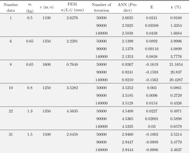
sam-ples in the test set are different in different training cycles. For example, when the training cycle is decreased from 9x10⁴ to 5x10⁴ for test samples of (1, 6, 10 and 22), the error rate has been de-creased between 0.1-0.4%, while for the test sample 8 and 31 it has inde-creased of between 0.05-0.2 percent. Moreover, increasing of the training cycle from 9x10⁴ to 14x104 has reduced the error rate between 0.1-0.3% for 6, 8, and 31. However, for (1, 10, 22) it has increased by approximately 0.2-0.3%. The reason of this behaviour is the learning performance of each example in training set can be different for different training cycles. For some examples, learning can be completed at the be-ginning of the training process, but it will continue until the specified tolerance of MSE is satisfied. In this case, the learning performance at the beginning of the training process with a very low error rate may decrease by increasing the error rate gradually. What is important for the network is not only to learn an example well, but also is to learn generally for all samples at low error rates. The other analyses made for all the other pairs in the test sample set have showed that similar results are valid.
Number data
mp
(kg) vp(m/s)
FEM
wz(L,t)(mm)
Number of iteration
ANN
(Pre-dict) E εt (%)
1 0.5 1100 2.6276 50000 2.6035 0.0241 0.9168
90000 2.5925 0.03508 1.3354
140000 2.5838 0.0438 1.6684
6 0.65 1350 2.2291 50000 2.1399 0.0892 3.9996
90000 2.1379 0.09116 4.0899
140000 2.1353 0.0838 3.7776
8 0.65 1600 0.7648 50000 0.9267 -0.1619 21.1654
90000 0.9241 -0.1593 20.837
140000 0.9210 -0.1562 20.4287
10 0.8 1250 3.5282 50000 3.5252 0.003 0.0861
90000 3.5185 0.0096 0.2729
140000 3.5128 0.0154 0.4326
22 1.3 1350 4.5635 50000 4.5408 0.0227 0.4971
90000 4.5365 0.02691 0.5898
140000 4.5335 0.03 0.6579
31 1.5 1500 2.8458 50000 2.9460 -0.1002 3.5214
90000 2.9447 -0.0989 3.4779
140000 2.9444 -0.0986 3.4637
Table 6: The performance of the ANN for different training round.
the third column shows the exit velocity of the projectile, the fourth column shows the value of the amount of muzzle displacement calculated using FEM, the fifth column shows muzzle displacements predicted using ANN, the sixth column shows the difference between the actual value and the ex-pected value, that is to say the error term, and the last column shows the relative error.
For each example in the test set, relative error is calculated as follows:
e =t E 100
B (32)
The data reported in Table 7 show that relative error is usually below 5%. The only exception is observed in the test set example 8, where the expected value was 0.7648 for a projectile mass of
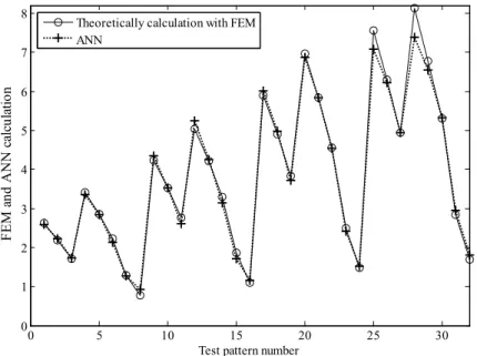
mp=0.65 kg and projectile exit velocity of 1600 m/s, but the ANN predicted a value of 0.9241. The relative error in this case was 20%. However, the relative errors for the rest of the test set examples show that overall the learning was very successful. Figure 8 shows the expected amount of muzzle displacement according to the theory and the amount predicted by the ANN.
Figure 8: FEM and ANN calculation for 35 mm anti-aircraft barrel tip deflection.
In this study, during the firing of a gun barrel, the displacement at the end of a barrel was es-timated by the artificial neural network. The obtained values were compared with the FEM model. The performance of the GDR algorithm used in design of ANN was compared with scaled conjugate gradient learning algorithm (SCH) used in literature. A comparison of the two algorithms GDR and SCH is given in Table 8, for the number of neurons in the hidden layer of the neural network from 3 to 8, and two different training cycle (9x10⁴, 14x104). After training is completed, as shown in table, the result of the testing of the samples contained in the test kit was obtained at the lowest average error, for 6 processing elements in middle layer and training cycle 9x10⁴.
0 5 10 15 20 25 30
0 1 2 3 4 5 6 7 8
Test pattern number
FE
M
a
nd
A
N
N
c
al
cu
la
tio
n
Number data mp (kg) vp(m/s) FEM
wz(L,t)(mm)
ANN (Predict) E εt (%)
1 0.5 1100 2.6276 2.5925 0.03508 1.3354
2 0.5 1250 2.1836 2.2209 -0.0373 1.7113
3 0.5 1350 1.7060 1.7381 -0.0321 1.8844
4 0.65 1000 3.4191 3.3510 0.06805 1.9905
5 0.65 1250 2.8525 2.8293 0.02315 0.8117
6 0.65 1350 2.2291 2.1379 0.09116 4.0899
7 0.65 1500 1.2907 1.2713 0.01939 1.5025
8 0.65 1600 0.7648 0.9241 -0.1593 20.837
9 0.8 1100 4.2427 4.3564 -0.1137 2.6820
10 0.8 1250 3.5282 3.5185 0.0096 0.2729
11 0.8 1350 2.7577 2.6084 0.14926 5.4125
12 0.95 1000 5.0390 5.2533 -0.2143 4.2535
13 0.95 1250 4.2108 4.2491 -0.0383 0.9096
14 0.95 1350 3.2922 3.1429 0.14922 4.5327
15 0.95 1500 1.8614 1.7079 0.15348 8.2456
16 0.95 1600 1.0944 1.1496 -0.0552 5.0462
17 1.1 1100 5.8881 6.0129 -0.1248 2.1199
18 1.1 1250 4.9006 4.9711 -0.0705 1.4390
19 1.1 1350 3.8328 3.7259 0.10687 2.7884
20 1.3 1000 6.9635 6.8682 0.09527 1.3682
21 1.3 1250 5.8320 5.8409 -0.0089 0.1528
22 1.3 1350 4.5635 4.5365 0.02691 0.5898
23 1.3 1500 2.4884 2.4249 0.06345 2.5500
24 1.3 1600 1.4744 1.5237 -0.0493 3.3444
25 1.4 1100 7.5654 7.0859 0.4794 6.3368
26 1.4 1250 6.3029 6.2149 0.0879 1.3951
27 1.4 1350 4.9334 4.9370 -0.0036 0.0738
28 1.5 1100 8.1318 7.3832 0.7485 9.2047
29 1.5 1250 6.7774 6.5428 0.2345 3.4610
30 1.5 1350 5.3063 5.3230 -0.0167 0.3150
31 1.5 1500 2.8458 2.9447 -0.0989 3.4779
32 1.5 1600 1.6993 1.8081 -0.1088 6.4078
Table 7: The testing set for 35 mm anti-aircraft cannon barrel and comparison of results.
single network topology that can represent all the engineering problems. The determination of net-work topology depends on the type of the problem, and the best netnet-work topology that will repre-sent the problem should be determined by designers using some trial and error methods. Therefore, a large number of neuron does not mean that it will certainly represent the problem well. Likewise, possession of a small number of neuron does not mean that the representation of problem is weak.
Algorithm
Number of neurons
Training
cycle. Training data Test data
MSE x
10-4 R2 error (%) Average MSE R2 error (%) Average
GDR 3 9x10⁴ 170.819 0.92015 11.8485 0.13000 0.99301 1.03567
GDR 3 14x104 170.853 0.92015 11.84856 0.13000 0.99301 1.03567
GDR 4 9x10⁴ 61.1896 0.97139 0.00314 0.43018 0.97689 7.66544
GDR 4 14x104 60.7863 0.97161 0.15147 0.42689 0.97707 7.51316
GDR 5 9x10⁴ 8.04889 0.99623 1.60089 0.11297 0.99393 2.72106
GDR 5 14x104 7.84242 0.99633 1.25377 0.13243 0.99288 3.15141
GDR 6 9x10⁴ 8.25235 0.99613 0.52192 0.03767 0.99797 0.09512
GDR 6 14x104 8.11695 0.99620 0.22156 0.03792 0.99796 0.19779
GDR 7 9x10⁴ 8.09059 09.9621 0.08644 1.85827 0.90020 12.82969
GDR 7 14x104 7.86834 0.99632 0.00328 1.61409 0.91331 13.21768
GDR 8 9x10⁴ 4.50216 0.99789 0.13103 16.22256 0.12881 18.60012
GDR 8 14x104 4.46487 0.99791 0.07493 16.43801 0.11724 18.87232
SCG 3 9x10⁴ 125.311 0.93015 10.8385 0.115280 0.99589 1.25963
SCG 3 14x104 109.103 0.92015 10.81258 0.125698 0.99457 1.35962
SCG 4 9x10⁴ 72.2589 0.97139 0.00418 0.58692 0.98529 6.95862
SCG 4 14x104 58.1936 0.99161 0.05637 0.40259 0.98301 7.02569
SCG 5 9x10⁴ 8.12569 0.99221 1.70283 0.20569 0.98697 202596
SCG 5 14x104 7.69253 0.99263 1.03698 0.1502 0.98995 3.32569
SCG 6 9x10⁴ 6.25987 0.99301 0.69583 0.06952 0.99105 0.09235
SCG 6 14x104 7.16391 0.99345 0.23594 0.04201 0.99304 0.12569
SCG 7 9x10⁴ 7.09059 09.9477 0.06965 1.52589 0.92038 10.2596
SCG 7 14x104 6.98696 0.99405 0.002589 1.32569 0.91658 11.1258
SCG 8 9x10⁴ 6.97652 0.99258 0.09687 15.2584 0.10881 13.60209
SCG 8 14x104 6.91256 0.99013 0.05896 15.2648 0.12724 13.23546
Table 8. Statistical data for the barrel tip displacement using two different algorithms.
5 CONCLUSION
weight and chemical content. This means that projectiles in different types of ammunition have different masses and muzzle exit velocities. Thus, muzzle behaviour during shooting varies by the type of ammunition used. The most important parameters affecting a weapon system’s dynamics are the projectile-mass, acceleration, and exit velocity.
The purpose of this study is to develop an artificial neural network to predict the amount of muzzle displacement, which is due to the force created by a projectile accelerating inside the barrel, and which reduces the shooting accuracy of a weapon system. Using the proposed method, one can determine the amount of muzzle displacement prior to shooting. In this method, the projectile mass and exit velocity are used as the input parameters of the neural network, while the amount of muz-zle displacement wz(x=L,t)is the output of the model. A training set is created to characterize the problem consisting of 25 examples from the problem space. At the end of the training process, which consisted of 90,000 training rounds, both the MSE and the individual errors E for the exam-ples in the training set were reduced to a very low level. The test set prepared to test the artificial neural network consisted of 32 examples covering the training space. Relative errors for some of the examples (Test pattern numbers 21, 27, and 30) were between 0.1- 0.2%, corresponding to about 0.009 mm, which is negligible for engineering purposes. In some of the test set examples (15 and 24), on the other hand, the relative error was about 8-9%, corresponding to a miscalculation of 0.15-0.7 mm. Only in one test set example (Test pattern number 8), the error was about 20%.
The method developed in this study makes it possible to examine the effect of different types of ammunition on the barrel using computers and eliminates the need for time consuming and costly tests. In addition, by integrating an artificial neural network trained according to barrel character-istics to the software, which is controlling barrel position, the shooting accuracy and strike power of the weapon system can be increased by simply adjusting the initial position of the barrel. This would make it possible to design weapons that are lighter and more effective against targets. The velocity of a projectile inside the barrel varies by time and forces the barrel to change its natural frequencies continuously. This means that for different projectiles and muzzle velocities, different vibration modes are created in the barrel. For example, the muzzle displacement value is positive at some muzzle velocities, and negative at others. In addition, predicting the amount of muzzle displacement in a weapon barrel may not be sufficient sometimes, predicting the angle of inclination of the barrel may also be required. The neural network modelled in this study does not require many complex systems to make prediction, but an artificial neural network with at least two hid-den layers is required only, and a preparation of a larger training set that represents the problem space are needed to predict both positive and negative muzzle displacements. Using the proposed method may help engineers in improving the target accuracy of a weapon system.
References
Alexander, E.J., 2007. AGS Gun and Projectile Dynamic Modeling Correlation to Test Data Branch Manager , Applied Mechanics. US Army Armament Syst. Div. 480–496.
Altınkaya, H., Orak, İ.M., Esen, İ., 2014. Artificial neural network application for modeling the rail rolling process. Expert Syst. Appl. 41, 7135–7146. doi:10.1016/j.eswa.2014.06.014
Balla, J., 2011. Dynamics of mounted automatic cannon on track vehicle. Int. J. Math. Model. Methods Appl. Sci. 5. Cay, Y., 2013. Prediction of a gasoline engine performance with artificial neural network. Fuel 111, 324–331. doi:10.1016/j.fuel.2012.12.040
Cifuentes, A.O., 1989. Dynamic response of a beam excited by a moving mass. Finite Elem. Anal. Des. 5, 237–246. doi:10.1016/0168-874X(89)90046-2
Clough R.W; Penzien J., 2003. Dynamics of Structures, Dynamics of Structures. doi:10.1002/9781118599792
Czarnigowski, J., 2010. A neural network model-based observer for idle speed control of ignition in SI engine. Eng. Appl. Artif. Intell. 23, 1–7. doi:10.1016/j.engappai.2009.09.008
Dehestani, M., Mofid, M., Vafai, A., 2009. Investigation of critical influential speed for moving mass problems on beams. Appl. Math. Model. 33, 3885–3895. doi:10.1016/j.apm.2009.01.003
Düğenci, M., Aydemir, A., Esen, İ., Aydın, M.E., 2015. Creep modelling of polypropylenes using artificial neural networks trained with Bee algorithms. Eng. Appl. Artif. Intell. 45, 71–79. doi:10.1016/j.engappai.2015.06.016
Esen, I., 2011. Dynamic response of a beam due to an accelerating moving mass using moving finite element approximation. Math. Comput. Appl. 16, 171–182.
Esen, İ., 2015. A new FEM procedure for transverse and longitudinal vibration analysis of thin rectangular plates subjected to a variable velocity moving load along an arbitrary trajectory. Lat. Am. J. Solids Struct. 12, 808–830. Esen, İ., 2013. A new finite element for transverse vibration of rectangular thin plates under a moving mass. Finite Elem. Anal. Des. 66, 26–35. doi:10.1016/j.finel.2012.11.005
Esen, İ., Koç, M.A., 2015a. Optimization of a passive vibration absorber for a barrel using the genetic algorithm. Expert Syst. Appl. 42, 894–905. doi:10.1016/j.eswa.2014.08.038
Esen, İ., Koç, M.A., 2015b. Dynamic response of a 120 mm smoothbore tank barrel during horizontal and inclined firing positions. Lat. Am. J. Solids Struct. 12, 1462–1486.
Esmailzadeh, E., Jalili, N., 2003. Vehicle–passenger–structure interaction of uniform bridges traversed by moving vehicles. J. Sound Vib. 260, 611–635. doi:10.1016/S0022-460X(02)00960-4
Hosseini, M., Dalvand, A., 2014. Neural Network Approach for Estimation of Penetration Depth in Concrete Targets by Ogive-nose Steel Projectiles. Lat. Am. J. Solids Struct. 12, 492–506.
Kadivar, M.H., Mohebpour, S.R., 1998. Finite element dynamic analysis of unsymmetric composite laminated beams with shear effect and rotary inertia under the action of moving loads. Finite Elem. Anal. Des. 29, 259–273. doi:10.1016/S0168-874X(98)00024-9
Kahya, V., 2012. Dynamic analysis of laminated composite beams under moving loads using finite element method. Nucl. Eng. Des. 243, 41–48. doi:10.1016/j.nucengdes.2011.12.015
Kathe, E., 1997. Design and validation of a gun barrel vibration absorber. New York.
Koide, R.M., Ferreira, A.P.C.S., Luersen, M.A., 2014. Laminated Composites Buckling Analysis Using Lamination Parameters, Neural Networks and Support Vector Regression. Lat. Am. J. Solids Struct. 12, 271–294.
L. Fryba, 1999. Vibration solids and structures under moving loads. Thomas Telford House.
Lagaros, N.D., Papadrakakis, M., 2012. Neural network based prediction schemes of the non-linear seismic response of 3D buildings. Adv. Eng. Softw. 44, 92–115. doi:10.1016/j.advengsoft.2011.05.033
Lee, H.P., 1996. Transverse vibration of a Timoshenko beam acted on by an accelerating mass. Appl. Acoust. 47, 319–330. doi:10.1016/0003-682X(95)00067-J
Littlefield, A., Kathe, E., Messier, R., Olsen, K., 2002. Gun barrel vibration absorber to increase accuracy. New York.