Clustering stability and ground truth: numerical experiments
Maria José Amorim Mathematical Department
ISEL and ISCTE-IUL Lisbon, Portugal
Margarida G. M. S. Cardoso
Business Research Unit and Department of Quantitative Methods for Management and Economics. ISCTE-IUL
Lisbon, Portugal
Abstract— Stability has been considered an important proper-ty for evaluating clustering solutions. Nevertheless, there are no conclusive studies on the relationship between this property and the capacity to recover clusters inherent to data (“ground truth”). This study focuses on this relationship, resorting to experiments on synthetic data generated under diverse scena-rios (controlling relevant factors) and experiments on real data sets. Stability is evaluated using a weighted cross-validation procedure. Indices of agreement (corrected for agreement by chance) are used both to assess stability and external valida-tion. The results obtained reveal a new perspective so far not mentioned in the literature. Despite the clear relationship be-tween stability and external validity when a broad range of scenarios is considered, the within-scenarios conclusions de-serve our special attention: faced with a specific clustering problem (as we do in practice), there is no significant relation-ship between clustering stability and the ability to recover data clusters
Keywords- Clustering; external validation; stability.
I. INTRODUCTION
Stability has been recognized as a desirable property of a clustering solution – e.g. [1]. A clustering solution is said to be stable if it remains fairly unchanged when the clustering process is subject to minor modifications such as, alternative parameterizations of the algorithm used, introducing noise in the data or considering different samples. In order to eva-luate stability, the agreement between the different cluster-ing results originated by such minor modifications is meas-ured. Several indices of agreement (IA), such as the adjusted Rand [2], are commonly used for this end.
Some authors warn of a possible misuse of the property of clustering stability noting that the goodness of this prop-erty in the evaluation of clustering results is not theoretically well founded: “While it is a reasonable requirement that an algorithm should demonstrate stability in general, it is not obvious that, among several stable algorithms, the one which is most stable leads to the best performance” –[3], p.1. Bubeck et al. express a similar concern: “While model selection based on clustering stability is widely used in prac-tice, its behavior is still not well-understood from a theoreti-cal point of view” - [4], p.436.
This study aims to contribute to clarify the role of sta-bility in the evaluation of clustering results. We focus on the relationship between clustering stability and its external
validity i.e. agreement with “ground truth” – the true clus-ters’ structures that are “a priori” known.
In order to obtain new insights we consider diverse ex-perimental scenarios and analyze diverse clustering results referred to 546 data sets. Synthetic data sets (540), generat-ed under 18 different scenarios, provide straightforward clustering external evaluation and enable to control for di-verse relevant factors such as the number of clusters, bal-ance and overlapping – e.g. [5], [6], [7]. The use of 6 real data sets from the UCI Machine Learning Repository [8], complements the experimental analysis.
II. ON CLUSTERING STABILITY A. Why stabilty?
Clustering stability, along with cohesion-separation, are commonly referred as desirable properties of a clustering solution. Cohesion-separation is intrinsically related with the concept of clustering and it can be related with the clus-ters' external validity - Milligan and Cooper [5] and Ven-dramin [6].
The value of stability is clearly related with the need to provide a useful clustering solution, since an inconsistent one would hardly serve practical purposes. On the other hand, the theoretical value of stability is yet to be unders-tood.
Literature contributions on stability are discussed in Luxburg [9] and Ben-David and Luxburg [3], for example. These are specifically related with the capacity to recover the "right" number of clusters and to K-Means results. Another perspective of stability is offered in [10] by mea-suring the consistency with which a particular cluster ap-pears in replicated clustering - cluster-wise stability.
The lack of a systematical relationship between clusters validity and stability is occasionally pointed out by diverse studies - e.g [11]. Thus, a systematical study of the relation-ship between stability and clustering external validity is in order.
B. Cross-Validation
In order to evaluate clustering stability cross-validation can be used. Cross-validation referred to unsupervised
anal-ysis, as described in [12], can be summarized into 5 main steps- Table 1.
TABLE 1. GENERAL CROSS-VALIDATION PROCEDURE
Step Action Output
1 Perform training-test Samplesplit
Training and test samples 2 Cluster training sample
Clusters in the training
sample 3
Build a classifier using the training sample supervisedby clusters' labels;
use theclassifier in the test sample.
Classes in the test sample 4 Cluster the test sample Clusters in the test
sample 5
Obtain a contingency tablebetween clusters and classesin the test sample
and calculate indices.
Indices of agree-ment values, indicators
of stability This clustering cross-validation procedure deserves, however, some remarks:
Referring to step 3 [13] point out that “by selecting an inappropriate classifier, one can artificially in-crease the discrepancy between solutions (…) the identification of optimal classifiers by analytical means seems unattainable. Therefore, we have to resort to potentially suboptimal classifiers in prac-tical applications”, (p.1304-1305);
In addition, the train-test split (step 1) requires suf-ficient sample size.
In this work, we resort to the weighted cross-validation procedure proposed in [11] to evaluate the stability of clus-tering solutions. The “weighted training sample” considers unit weights for training observations (50% in the data sets considered) and almost zero weights to the remaining (test) observations. The “weighted test sample” reverses this weights’ allocation. The use of weighted samples over-comes the need for selecting a classifier when performing cross-validation. Furthermore, sample dimension is not a severe limitation for implementing clustering stability eval-uation, since the Indices of agreement values are based on the entire (weighted) sample, and not in a holdout sample.
C. Adjusted agreement between partitions
In order to measure the agreement between two parti-tions we can resort to indices of agreement (𝐼𝐴). In the lite-rature, multiple 𝐼𝐴 can be found – e.g. [14], [15]. They are generally quantified based on the cells values of the contin-gency table between the two partitions being compared - 𝑃𝐾 and 𝑃𝑄with 𝐾and 𝑄 clusters (respectively).
Among the 𝐼𝐴, the Rand index (𝑅𝑎𝑛𝑑) is, perhaps, the most well-known - [16]. 𝑅𝑎𝑛𝑑 𝑃𝐾, 𝑃𝑄 = 𝑛 2 + 2 𝑛𝑘𝑞 2 − 𝑛𝑘+ 2 − 𝑛+𝑞 2 𝑄 𝑞=1 𝐾 𝑘=1 𝑄 𝑞=1 𝐾 𝑘=1 𝑛 . (1)
Where 𝑛𝑘𝑞 are the cells values of the contingency table, and 𝑛𝑘+ and 𝑛+𝑞 are the corresponding row totals and col-umn totals, respectively.
It quantifies the proportion of pairs of observations that both partitions agree to join in a group or to separate into different groups. Since agreement between partitions can occur by chance, [2] propose an adjusted version of𝑅𝑎𝑛𝑑 us-ing its expected value under the hypothesis of agreement by chance (𝐻𝑜): 𝐸𝐻0 𝑛2𝑘𝑞 𝑄 𝑞=1 𝐾 𝑘=1 = 𝑛𝑘+ 2 × 𝑛+𝑞 2 𝑄 𝑞=1 𝐾 𝑘=1 𝑛2 . (2)
Then this 𝐼𝐴 is adjusted according with the general for-mula: 𝐼𝐴𝑎 𝑃𝐾, 𝑃𝑄 = 𝐼𝐴 𝑃𝐾, 𝑃𝑄 − 𝐸 𝐻0 𝐼𝐴 𝑃𝐾, 𝑃𝑄 𝑀𝑎𝑥 𝐼𝐴 𝑃𝐾, 𝑃𝑄 − 𝐸 𝐻0 𝐼𝐴 𝑃𝐾, 𝑃𝑄 . (3)
The adjusted index 𝐼𝐴𝑎 is thus null when agreement between partitions occurs by chance. Some 𝐼𝐴 are based on the concepts of entropy and information. Among these𝐼𝐴, Mutual Information (𝑀𝐼) is particularly well-known:
𝑀𝐼 𝑃𝐾, 𝑃𝑄 = 𝑛𝑘𝑞 𝑛 log 𝑛𝑘𝑞 𝑛𝑘+𝑛+𝑞 𝑛 𝑄 𝑞=1 𝐾 𝑘=1 . (4)
Vinh et al., [14], advocate a strategy similar to that of [2] to adjust 𝑀𝐼 for agreement by chance. These authors also advocate the use of a particular mutual information form resorting to joint entropy 𝐻 𝑃𝐾, 𝑃𝑄 – ([17], [18]):
𝑀𝐼𝐻 𝑃𝐾, 𝑃𝑄 =𝑀𝐼 𝑃𝐾, 𝑃𝑄 𝐻 𝑃𝐾, 𝑃𝑄 , (5) where 𝐻 𝑃𝐾, 𝑃𝑄 = − 𝑛𝑘𝑞 𝑛 log 𝑛𝑘𝑞 𝑛 𝑄 𝑞=1 𝐾 𝑘=1 . (6)
In order to investigate agreement between two parti-tionswe resort to the adjusted indices 𝑅𝑎𝑛𝑑𝑎 𝑃𝐾, 𝑃𝑄 and𝑀𝐼𝐻𝑎 𝑃𝐾, 𝑃𝑄 . They offer different perspectives on agreement – paired agreement and simple agreement [19]. These views are meant to provide useful insights when re-ferring to external validation (comparison between the clus-tering solution and the “true” cluster structure) or to the evaluation of stability (comparison between two clustering solutions deriving from minor modifications in the cluster-ing process).
III. NUMERICAL EXPERIMENTS A. Synthetic data
The pioneer study of Milligan and Cooper, [5], estab-lished the use of synthetic data to support the external vali-dation of clustering structures. In this general setting, clus-tering solutions are to be compared with a priori known classes associated with the generated data sets. Since then, several works referring to external validation of clustering solutions have developed this line of work trying to over-come some drawbacks of this first study such as using the “right number of clusters” to quantify external validity is limited in scope, [6]. In addition, overlap between clusters should be properly quantified on the generation of experi-mental data sets [20].
The present research considers three main design factors for the generation of synthetic data sets:
balance (1- clusters are balanced having equal or very similar numbers of observations; 2- clusters are unbalanced)
number of clusters (K=2, 3,4)
clusters separation (1- poor; 2-moderate; 3- good). The 18 resulting scenarios are named after the previous coding – for example, the scenario with balanced clusters (1), 3 clusters (3) and moderate separation (2) is termed “132”.
The first design factor is operationalized as follows: ba-lanced settings have classes with similar dimensions and for unbalanced settings classes have the following a priori probabilities orweights: a) 0.30 and 0.7 when K=2; b) 0.6, 0.3 and 0.1 when K=3; c) 0.5, 0.25, 0.15 and 0.10 when K=4.
The increasing number of clusters is associated with in-creasing number of variables (2, 3 and 4 latent groups with 2, 3 and 4 Gaussian distributed variables) and, in order to deal with this increasing complexity, we consider data sets with 500, 800 and 1100 observations, respectively.
The following measure of overlap between the classes 𝑘 and 𝑘’ is adopted, [21]:
ωkk′ = ωk|k′ + ωk′|k , (7) where 𝜔k′ |kis the misclassification probability that the ran-dom variable 𝑋originated from the kth component is mista-kenly assigned to the k’th component and 𝜔k|k′ is defined similarly.
In order to generate the datasets within the scenarios, we capitalize on the recent contribution in [21] and use the R MixSimpackage to generate structured data according to the finite Gaussian mixture model:
𝜆𝑘𝜙(𝑥; 𝜇𝑘, 𝛴𝑘) 𝐾
𝑘=1
, (8)
where 𝜙(𝑥; 𝜇𝑘, Σ𝑘) is a multivariate Gaussian density of the kth component with mean vector𝜇𝑘 and covariance matrix Σ𝑘. Therefore,
ωk′ |k = 𝑃 λk′ϕ x; μk′, Σk′ >
λkϕ x; 𝜇𝑘, Σk |𝑥 ~𝑁𝑝 μk, Σk .
(9)
Based on this measure, we consider three degrees of overlap in the experimental scenarios: 1) ωkk′ is around 0.6 for poorly separated clusters; 2) ωkk′ is around 0.15 for moderately separated; 3) ωkk′ is around 0.02 for well sepa-rated classes. These thresholds are indicated in [21].
For each of the referred 18 scenarios, we generate 30 da-tasets and run our experiments by:
clustering each data set;
evaluating stability of the clustering solution (seeII.A and II.C);
evaluating clustering external validity based on the
a priori known classes (see II.C);
correlating results from stability and external valid-ity to assess the role of the stabilvalid-ity property. The Rmixmod package is used for clustering purposes [22]. EM algorithm is found to be particularly suited for the clustering tasks at hand, since the data generated follow a finite Gaussian mixture model. We use the general Gaussian mixture model - [PKLKBK] in [23].
The first results obtained are summarized in Table 2 and Table 3. They reveal the pertinence of the design fac-tors:stability and external validity increase with the increase in separation, the 𝐼𝐴 being close to zero when separation is poor and near one when well separated clusters are consi-dered. In general, the adjusted Rand index and mutual in-formation values illustrate the same underlying reality, al-though the 𝑀𝐼𝐻𝑎 values provide a more conservative view of the degree of agreement between two partitions.
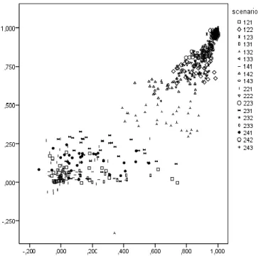
The general results referring to the relationship between stability and agreement with ground truth (inter experimen-tal scenarios), are illustrated in Figure1 and Figure 2. The corresponding Pearson correlation values are 0.958 and 0.933, respectively, indicating a high linear correlation be-tween stability and external validity (both measured by 𝑀𝐼𝐻𝑎in Figure1 and 𝑅𝑎𝑛𝑑𝑎inFigure 2. These results corro-borate the general theory on the relevance of the property of stability in the evaluation of clustering solutions.
A completely different view is however provided intra-scenarios,yielding very low correlations between stability and external validity – see Table 4. Within a specific scena-rio - the “real deal” for any clustering analysis practitioner - the correlation between external validity and stability is negligible. Both the adjusted Rand and the adjusted Mutual Information lead to the same conclusion. Only two excep-tions contradict this rule: scenarios “232” and “143”.
B. Real data
The agreement between ground truth and stability is also subject to inspection in six data sets of the UCI Machine Learning Repository [8] – see Table 5 for a brief summary of these data sets. In addition to the design factors previous-ly
TABLE 2 - ADJUSTED RAND INDEX VALUES CORRESPONDING TO EXTERNAL VALIDITY AND TO STABILITY (VALUES
AVERAGED OVER 30 DATASETS). 𝑹𝒂𝒏𝒅𝐚
External validity Stability
K=2 K=3 K=4 K=2 K=3 K=4 Balanced Poor 0.055 0.038 0.041 0.111 0.118 0.085 Moder. 0.728 0.388 0.624 0.865 0.652 0.688 Good 0.963 0.943 0.855 0.987 0.979 0.918 Unbalanced Poor 0.097 0.211 0.133 0.053 0.280 0.166 Moder. 0.765 0.690 0.820 0.864 0.822 0.898 Good 0.962 0.980 0.887 0.981 0.991 0.949
TABLE 3 - MUTUAL INFORMATION ADJUSTED VALUESCORRESPONDING TO EXTERNAL VALIDITY AND TO
STABILITY (VALUES AVERAGED OVER 30 DATASETS). 𝑴𝑰𝑯𝒂
External validity Stability
K=2 K=3 K=2 K=3 K=2 K=3 Balanced Poor 0.046 0.024 0.031 0.073 0.054 0.073 Moder. 0.458 0.263 0.449 0.700 0.465 0.578 Good 0.865 0.832 0.707 0.949 0.931 0.833 Unbalanced Poor 0.048 0.093 0.070 0.036 0.189 0.124 Moder. 0.477 0.440 0.569 0.660 0.613 0.732 Good 0.850 0.920 0.694 0.922 0.957 0.840
TABLE 4 - INTRA-SCENARIOS PEARSON CORRELATIONS BETWEEN STABILITY AND AGREEMENT FOR SYNTHETIC DATA.
𝑴𝑰𝑯𝒂 𝑹𝒂𝒏𝒅𝒂 K=2 K=3 K=4 K=2 K=3 K=4 Balanced Poor 0.143 -0.018 -0.129 -0.079 -0.155 -0.303 Mod. 0.122 0.264 -0.015 0.068 0.215 0.111 Good 0.084 0.222 0.527 0.046 0.177 0.624 Unbalanced Poor 0.329 0.126 0.172 0.367 -0.42 -0.079 Mod. -0.003 0.593 0.084 0.085 0.666 0.084 Good -0.151 0.272 0.245 -0.084 0.159 0.218
considered, we also quantify normalized entropy (ranging from 0 to 1 that indicates classes’ uniform distribution).
Since the real data sets are diverse, we attempt to recov-er their clustrecov-ering structures resorting to diffrecov-erent clustrecov-ering
algorithms - namely the Hartigan K-Means (KM) algorithm [24], the Expectation Maximization (EM) [25] and the Sto-chastic EM (SEM) [26]. We resort to the EM and the SEM algorithms implemented in the Rmixmod package using the general Gaussian mixture model - [PKLKBK] in [23].
FIGURE1. INTER-SCENARIOS PEARSON CORRELATION BETWEEN STABILITY (YY’) AND AGREEMENT WITH GROUND
FIGURE 2. INTER-SCENARIOS PEARSON CORRELATION BETWEEN STABILITY (YY’) AND AGREEMENT WITH GROUND
TABLE 5 - REAL DATA SETS
Data set n Features Classes Normalized
Entropy Overlapping Liver Disorders 345 6 C1 (145) C2 (200) 0.982 0.016 Wholesales 440 6 C1 (298) C2 (142) 0.907 0.111 Iris 150 4 Setosa (50) Versicolor (50) Virginica (50) 1.585 0.518 Wine recognition data 178 12 C1 (59) C2 (71) C3 (48) 1.567 0.002 Cars Silhouette 846 18 Bus (218) Saab (217) Opel (212) Van (199) 1.999067 0.044 User Modeling 258 5 Very-low (24) Low (83) Middle (88) High (63) 1.871 0.028
According to the results obtained (Table 6), the clustering solutions are generally stable,while agreement with ground truth varies appreciably. Thus, there is no relationship be-tween stability and agreement with ground truth, the rela-tionship under study appearing to be mainly dependent of the data set at hand.
IV. CONTRIBUTIONS AND PERSPECTIVES
In this work we analyze the pertinence of using stability in the evaluation of a clustering solution. In particular, we question the following: does the consistency of a clustering solution (resisting minor modifications of the clustering process) provide indication towards a greater agreement with the “ground truth” (true structure) of the data?
In order to address this issue, we design an experiment in which 540 synthetic data sets are generated under 18 different scenarios. Design factors considered are the num-ber of clusters, their balance and overlap. In addition, differ-ent sample sizes and space dimensions are considered.
Through the use of weighted cross-validation, we enable the analysis of stability, [11]. We resort to adjusted indices of agreement (excluding agreement by chance) to measure agreement between two clustering solutions and also be-tween a clustering solution and the “true” classes: we specif-ically use a simple index of agreement (IA) - the adjusted Mutual Information, [14] - and a paired IA - the adjusted Rand index [2].
A macro-view of the results does not contradict the cur-rent theory - there is a strong correlation between stability and external validity when the aggregate results are consi-dered (all scenarios’ results). However, when it comes to perform clustering analysis within a specific experimental scenario, what can we say about the same correlation? The conclusions derived in this study support the previously referred concerns referring to the relationship between sta-bility and agreement
TABLE 6.- STABILITY AND GROUND TRUTH FOR REAL DATA
Data set rithm
Algo-Agreement with ground truth
Stability on
Weighted-train/test
Randa MIHa Randa MIHa
Liver KM -0.005 -0.001 0.943 0.786 EM -0.009 0.002 0.960 0.844 SEM -0.010 0.002 0.987 0.933 Whole-sales KM 0.564 0.311 -0.032 0.005 EM 0.427 0.245 0.843 0.609 SEM 0.427 0.251 0.851 0.621 Iris KM 0.730 0.608 0.924 0.786 EM 0.834 0.692 0.478 0.486 SEM 0.834 0.699 0.478 0.486 Wine recogni-tion data KM 0.352 0.264 0.760 0.615 EM 0.915 0.805 0.802 0.691 SEM 0.915 0.805 0.833 0.719 Cars KM 0.126 0.099 0.651 0.552 EM 0.143 0.102 0.601 0.521 SEM 0.144 0.103 0.604 0.526 User Modeling KM 0.189 -0.217 0.474 -0.126 EM 0.372 0.118 0.574 0.245 SEM 0.372 -0.131 0.531 -0.013 with ground truth – there is an insignificant correlation be-tween stability and external validity when it comes to a specific clustering problem.
Of course, it is still true that an unstable solution is, for this very reason, undesirable (otherwise which results should the practitioner consider?). However, in a specific clustering setting, there is clearly no credible link between the stability of a partition and its approximation to ground truth.
This work contributes with a new perspective for a better understanding of the relationship between clustering stabili-ty and its external validistabili-ty. To our knowledge, is the first time a study distinguishes between the macro view (all ex-perimental scenarios considered) and the micro view (consi-dering a specific clustering problem) and clearly differen-tiates the corresponding results.
In the future, stability results in discrete clustering should also be assessed and possible additional experimental factors (e.g. clusters’ entropy)may also be considered.
REFERENCES
1. Jain, A.K. and R.C. Dubes, Algorithms for clustering data. 1988: Englewood Cliffs, N.J.: Prentice Hall.
2. Hubert, L. and P. Arabie, “Comparing partitions”, Journal of Classification, Vol 2, 1985, pp. 193-218.
3. Ben-David, S. and U.V. Luxburg, ”Relating clustering stability to properties of cluster boundaries” in 21st Annual Conference on Learning Theory (COLT), Berlin: Springer, pp 379-390, July 2008.
4. Bubeck, S., M. Meila, and U. von Luxburg, “How the initialization affects the stability of the k-means algorithm” ESAIM: Probability and Statistics, Vol 16, 2012, pp. 436-452.
5. Milligan, G.W. and M.C. Cooper, “An examination of procedures for determining the number of clusters in a data set.” Psychometrika, Vol 50, Issue 2, 1985, pp. 159-179. 6. Vendramin, L., R.J. Campello, and E.R. Hruschka, “Relative
clustering validity criteria: A comparative overview” Statistical Analysis and Data Mining, Vol 3, Issue 4, 2010, pp. 209-235.
7. Chiang, M.M.-T. and B. Mirkin, “Intelligent Choice of the Number of Clusters in K-Means Clustering: An Experimental Study with Different Cluster Spreads” Journal of Classification, Vol 27, 2010, pp. 3-40.
8. Lichman, M. UCI Machine Learning Repository 2013; Available from: http://archive.ics.uci.edu/ml.
9. Luxburg, U.v., “Clustering Stability: An Overview” Machine Learning, Vol 2, issue 3, 2009, pp. 235-274.
10. Hennig, C., “Cluster-wise assessment of cluster stability” Computational Statistics & Data Analysis, Vol 52, 2007, pp. 258-271.
11. Cardoso, M.G., K. Faceli, and A.C. de Carvalho, Evaluation of Clustering Results: The Trade-off Bias-Variability, in Classification as a Tool for Research., Springer, pp. 201-208, 2010.
12. McIntyre, R.M. and R.K. Blashfield, “A nearest-centroid technique for evaluating the minimum-variance clustering procedure” Multivariate Behavioral Research, Vol 2, 1980, pp. 225-238.
13. Lange, T., et al., “Stability based validation of clustering solutions” Neural Computation, Vol 16, 2004, pp. 1299-1323.
14. Vinh, N.X., J. Epps, and J. Bailey, “Information theoretic measures for clusterings comparison: Variants, properties, normalization and correction for chance” The Journal of Machine Learning Research, Vol 11, 2010, pp. 2837-2854. 15. Warrens, M.J., “On similarity coefficients for 2× 2 tables and
correction for chance”, Psychometrika, Vol 73, Issue 3, 2008, pp. 487-502.
16. Rand, W.M., “Objective criteria for the evaluation of clustering methods”, Journal of the American Statistical Association, Vol 66, 1971, pp. 846-850.
17. Horibe, Y., “Entropy and correlation” Systems, Man and Cybernetics, IEEE Transactions, Vol 5, 1985, pp. 641-642. 18. Kraskov, A., et al., “Hierarchical clustering using mutual
information”, EPL (Europhysics Letters), Vol 70, Issue 2, 2005, pp. 278.
19. Cardoso, M.G.M.S. Clustering and Cross-Validation. in IASC 07 - Statistics for Data Mining, Learning and Knowledge Extraction, Aveiro, Portugal, August 2007 20. Steinley, D. and R. Henson, “OCLUS: an analytic method
for generating clusters with known overlap” Journal of Classification, Vol 22, Issue 2, 2005,pp. 221-250.
21. Maitra, R. and V. Melnykov, “Simulating data to study performance of finite mixture modeling and clustering algorithms” Journal of Computational and Graphical Statistics, Vol 19, 2010, pp. 354-376.
22. Lebret, R., et al.” Rmixmod: The r package of the model-based unsupervised, supervised and semi- supervised classification” 2012; Available from: http://cran.r-project.org/web/packages/Rmixmod/ index.html
23. Biernacki, C., et al.,” Model-Based Cluster and Discriminant Analysis with the MIXMOD Software” Computational Statistics and Data Analysis, Vol 51, 2006, pp. 587-600. 24. Hartigan, J.A., Clustering algorithms. 1975.
25. Dempster, A.P., N.M. Laird, and D.B. Rubin, “Maximum likelihood from incomplete data via the EM algorithm” Journal of the Royal Statistics Society. Series B (Methodological), Vol 39, 1977, pp. 1-38.
26. Celeux, G. and J. Diebolt, “The SEM Algorithm: A probabilistic teacher algorithm derived from the EM algorithm for the mixture problem” Computational Statistics Quarterly, Vol 2, 1985, pp. 73-8.