Optimal Control and Sensitivity Analysis of a Fractional Order TB Model

Published online in International Academic Press (www.IAPress.org)

Optimal Control and Sensitivity Analysis of a Fractional Order TB Model

Silv´erio Rosa

, Delfim F. M. Torres

1_{Department of Mathematics and Instituto de Telecomunicac¸˜oes (IT), University of Beira Interior, 6201-001 Covilh˜a, Portugal} 2_{Center for Research and Development in Mathematics and Applications (CIDMA), Department of Mathematics, University of Aveiro,}

3810-193 Aveiro, Portugal

Abstract A Caputo fractional-order mathematical model for the transmission dynamics of tuberculosis (TB) was recently

proposed in [Math. Model. Nat. Phenom. 13 (2018), no. 1, Art. 9]. Here, a sensitivity analysis of that model is done, showing the importance of accuracy of parameter values. A fractional optimal control (FOC) problem is then formulated and solved, with the rate of treatment as the control variable. Finally, a cost-effectiveness analysis is performed to assess the cost and the effectiveness of the control measures during the intervention, showing in which conditions FOC is useful with respect to classical (integer-order) optimal control.

Keywords Tuberculosis; Compartmental mathematical models; Fractional optimal control.

AMS 2010 subject classifications34A08, 49M05, 92C60 DOI:10.19139/soic-2310-5070-836

1. Introduction

Tuberculosis (TB) is an infectious disease caused by the bacterium Mycobacterium tuberculosis, which is usually spread through the air when people who have active TB in their lungs cough, spit, speak, or sneeze. TB is one of the top ten causes of death worldwide, which justifies the interest of researchers on the area: see, e.g., [17, 19, 23]. A good survey on optimal models of TB is presented in [20]. Delays are introduced in a TB model in [17], representing the time delay on the diagnosis and initiation of treatment of individuals with active TB infection. Optimal control strategies to minimize the cost of interventions, considering reinfection and post-exposure interventions, are investigated in [19]. In [15], the potential of two post-exposure interventions, treatment of early latent TB individuals and prophylactic treatment/vaccination of persistent latent TB individuals, is investigated. A mathematical model for TB is studied in [5] from the optimal control point of view, using a multiobjective optimization approach. For numerical simulations using TB real data from Angola, see [18]. In spite of the numerous works on tuberculosis, the literature on fractional-order mathematical models for TB is still scarce. In [21], it is proposed a multi-strain TB model with variable-order fractional derivatives and a numerical scheme to approximate the endemic solution, numerically, is developed. More recently, in 2018, a Caputo type fractional-order mathematical model for the transmission dynamics of tuberculosis was proposed, based on the nonlinear differential system studied in [25], and its stability is investigated [24]. Such model is here subject to fractional optimal control theory [4,7], and its usefulness to tackle a TB epidemic scenario discussed.

The paper is organized as follows. In Section2, we introduce the fractional-order TB model. The main results are then given in Section3: sensitivity analysis of the fractional TB model (Section3.1); fractional optimal control,

∗_{Correspondence to: Delfim F. M. Torres (Email: delfim@ua.pt). Department of Mathematics, University of Aveiro, 3810-193 Aveiro,}

cost-effectiveness and numerical simulations for the TB model (Sections3.2and3.3). We end with Section4of conclusions.

2. Fractional-order Tuberculosis Model

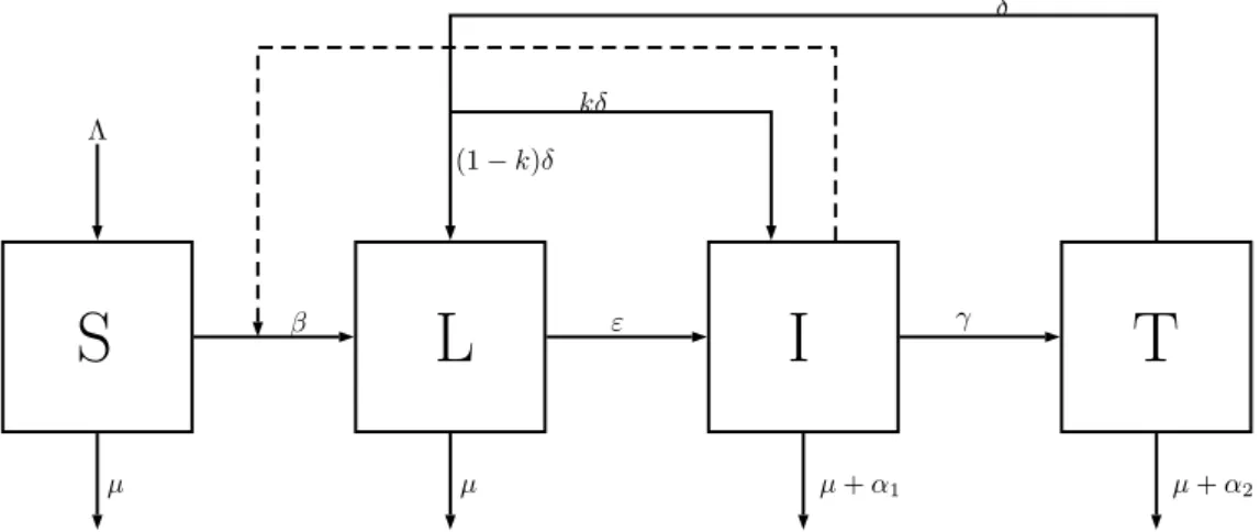
In this section, we consider a Caputo fractional-order tuberculosis (TB) model due to [24]. The model describes the dynamics of a population that is susceptible to infection by the Mycobacterium tuberculosis with incomplete treatment. The population consists of four compartments: susceptible individuals (S); latent individuals (L), which have been infected but are not infectious and do not show symptoms of the disease; infectious individuals (I), which have active TB, may transmit the infection, but are not under treatment; and infected individuals in treatment (T).

The susceptible population is increased by the recruitment of individuals into the population at a rate Λ. All individuals are exposed to natural death, at a constant rateµ. Deterministic continuous transitions between the compartments, also known as states, are used. Susceptible individuals acquire TB infection by the contact with infected individuals at a rateβI, where parameterβis the transmission coefficient. Individuals in the latent class,

L, become infectious at a rateε, and infectious individuals,I, start treatment at a rateγ. Treated individuals,T, leave their compartment at rateδ. After leaving the treatment compartment, an individual may enter compartment

L, due to the remainder of Mycobacterium tuberculosis, or compartment I, due to the failure of treatment. The parameterk,06k61, represents the failure of the treatment, wherek = 0means that all the treated individuals shall become latent, whilek = 1means that the treatment fails and all the treated individuals shall still be infectious. Infectious,I, and under treatment individuals,T, may suffer TB-induced death at the ratesα1andα2, respectively.

The Caputo fractional-order system of differential equations that describes the above assumptions is          C 0D α tS(t) = Λ− βI(t)S(t) − µS(t), C 0D α tL(t) = βI(t)S(t) + (1− k)δT (t) − (µ + ε)L(t), C 0D α tI(t) = εL(t) + kδT (t)− (µ + γ + α1)I(t), C 0D α tT (t) = γI(t)− (µ + δ + α2)T (t), (1) whereC 0D α

t denotes the left Caputo derivative of orderα∈ (0, 1][12,16]. Note that whenα = 1, the fractional

compartmental model (1) represents the classical TB model studied in [25]. In Figure1, one can find a diagram representing the model dynamics.

S

L

I

T

3. Main results

We begin by investigating the sensitiveness of the TB model (1), discussed in Section2, with respect to the variation of each one of its parameters.

3.1. Sensitivity analysis

One of the most significant thresholds when studying infectious disease models is the basic reproduction number [22]. The basic reproduction number for the TB model (1) is given by

R0= βεb3Λ

µb1b2b3− µδγ((1 − k)ε + kb1) (2)

withb1= µ + ε,b2= µ + γ + α1andb3= µ + δ + α2[25].

Now we perform a sensitivity analysis for the endemic threshold (2). Such analysis tells us how important each parameter is to disease transmission. This information is crucial not only for experimental design, but also to data assimilation and reduction of complex models [13]. Sensitivity analysis is commonly used to determine the robustness of model predictions to parameter values, since there are usually errors in collected data and presumed parameter values. It is used to discover parameters that have a high impact on the threshold R0 and should be

targeted by intervention strategies. More accurately, sensitivity indices’s allows us to measure the relative change in a variable when parameter changes. For that purpose we use the normalized forward sensitivity index of a variable, with respect to a given parameter, which is defined as the ratio of the relative change in the variable to the relative change in the parameter. If such variable is differentiable with respect to the parameter, then the sensitivity index is defined using partial derivatives.

Definition 1 (See [3,14])

The normalized forward sensitivity index of R0, which is differentiable with respect to a given parameterp, is

defined by ΥR0 p = ∂R0 ∂p p R0.

The values of the sensitivity indices for the parameters values of Table1, are presented in Table2.

Table 1. Values of the models’ parameters taken from [24,25].

Name Description Value

Λ Recruitment rate 792.8571

β Transmission coefficient 0.0005

µ Natural death rate 1/70

k Treatment failure rate 0.15

δ Rate at which treated individuals leave theTcompartment 1.5

ε Rate at which latent individualsLbecome infectious 0.00368

α1 TB-induced death rate for infectious individualsI 0.3 α2 TB-induced death rate for under treatment individualsT 0.05

Note that the sensitivity index may depend on several parameters of the system, but also can be constant, independent of any parameter. For example, ΥR0

Λ = +1, meaning that increasing (decreasing) Λ by a given

percentage increases (decreases) always R0 by that same percentage. The estimation of a sensitive parameter should be carefully done, since a small perturbation in such parameter leads to relevant quantitative changes. On the other hand, the estimation of a parameter with a rather small value for the sensitivity index does not require as much attention to estimate, because a small perturbation in that parameter leads to small changes [10]. According to our results in Table2, special attention should be paid to the estimation of the death rate,µ. In contrast, the rate at which individuals leave stateT,δ, does not require as much attention because of its low value of the sensitivity

Table 2. Sensitivity ofR0evaluated for the parameter values given in Table1.

Parameter Sensitivity index

µ −1.93223 ε +0.911803 γ −0.605532 α1 −0.376538 δ 0.0112215 α2 −0.0872783 Λ +1 k +0.100487 β +1

index. This is well illustrated in Figure2, where we can see in Figure2athe graphics of the number of infective with and without an increment of 15% for the parameterµ(most sensitive parameter), and in Figure2bwith identical comparison of graphics for parameterδ(less sensitive parameter).

time 0 0.5 1 1.5 2 2.5 3 3.5 4 4.5 5 150 200 250 300 350 400 450 500 Original µ Increased µ

(a) Impact of the variation ofµin the number of infective

individualsI(there is a visible difference).

time 0 0.5 1 1.5 2 2.5 3 3.5 4 4.5 5 150 200 250 300 350 400 450 500 Original δ Increased δ

(b) Impact of the variation ofδin the number of infective

individualsI(no visible difference).

Figure 2. Infected number of individuals predicted by the TB model (1) with original parameter values as in Table1and with

an increase of 15% of a specific parameter:µin (a) andδin (b).

Using the values of the parameters as proposed in [24], we obtain results very different from those that the authors present there. We noticed that the value of parameterµpresented in [24] (µ′= 0.143), the most sensitive one, is erroneous, being 10 times the correct value [25] and was not the value that authors’ used in the simulation. This particular case highlights the importance of the analysis we have carried out here.

3.2. Fractional optimal control

The circumstances on which variation of the variables of the model depend, may be controlled. In case of TB disease, the fraction of infectious individuals that is identified and put under treatment is one of the most commonly used. Therefore, the parameterγis, in what follows, replaced by a control variable. Consequently, we consider the following fractional optimal control problem: to minimize the number of infectious individuals and the cost of the control of the disease with the identification and treatment of the patients, that is,

min J (I(t), u(t)) =

∫ tf

0

with0 < B <∞, subject to the fractional control system          C 0D α tS(t) = Λ− βI(t)S(t) − µS(t) C 0D α tL(t) = βI(t)S(t) + (1− k)δT (t) − (µ + ε)L(t) C 0D α

tI(t) = εL(t) + kδT (t)− (µ + u(t) + α1)I(t)

C

0D α

tT (t) = u(t)I(t)− (µ + δ + α2)T (t)

(4)

and given initial conditions

S(0), L(0), I(0), T (0)>0. (5)

Here,ρis the maximum number of infectious individuals of the problem without control; and the control variable,

u, designate the fraction of individuals that is put under treatment. The set of admissible control functions is

Ω ={u(·) ∈ L∞(0, tf) : 06u(t)6umax,∀t ∈ [0, tf]} . (6)

Pontryagin’s maximum principle (PMP) for fractional optimal control can be used to solve the problem [1,2,8,9]. The Hamiltonian associated with our optimal control problem is

H = I + Bρ u2_{+ p}

1(Λ− βIS − µS)

+ p2(βIS + (1− k)δT − (µ + ε)L) + p3(εL + kδT − (µ + u + α1)I) + p4(uI− (µ + δ + α2)T );

the adjoint system uphold that the co-state variablespi(t),i = 1, . . . , 4, verify              tDα_tfp1(t) = µp1(t)− βI(t)(p1(t)− p2(t)), tD α tfp2(t) = (ε + µ)p2(t)− εp3(t), tD α tfp3(t) =−1 + (α1+ u(t) + µ)p3(t)− u(t)p4(t) + βS(t)(p1(t)− p2(t)), tD α tfp4(t) = (α2+ µ + δ) p4(t) + δ(k− 1)p2(t)− δkp3(t), (7)

which is a fractional system of right Riemann–Liouville fractional derivatives, tD

α

tf. In turn, the optimality

condition of PMP establishes that the optimal control is given by

u(t) = min { max { 0,(p3(t)− p4(t)) I(t) 2Bρ } , umax } . (8)

In addition, the following transversality conditions hold:

tD α₋₁ tf pi _tf= 0⇔tI 1_−α tf pi _tf= pi(tf) = 0, i = 1, . . . , 4, (9) wheretI 1_−α

tf is the right Riemann–Liouville fractional integral of order1− α.

3.3. Numerical results and cost-effectiveness of the fractional TB optimal control problem

The PMP is used to numerically solve the optimal control problem (3)–(6), as discussed in Section 3.2, in the classical (α = 1) and fractional (0 < α < 1) cases, using the predict-evaluate-correct-evaluate (PECE) method of Adams–Basforth–Moulton [6], implemented in MATLAB. First, we solve system (4) by the PECE procedure with initial values for the state variables given by Table3and a guess for the control over the time interval[0, tf], and obtain the values of the state variablesS,L,I andT. A change of variables is applied to the adjoint system (7) and to the transversality conditions (9), obtaining a left Riemann–Liouville fractional initial value problem. Such system is solved with the PECE procedure and the values of the co-state variablespi,i = 1, . . . , 4, are obtained.

The control is then updated by a convex combination of the previous control and the value computed according to (8). This procedure is repeated iteratively until the values of the controls at the previous iteration are very close to

the ones at the current iteration. The solutions of the classical problem (α = 1) where successfully confirmed by an algorithm that uses a classical forward-backward scheme, also implemented in MATLAB.

In our numerical experiments, we consider that the maximum number of infectious individuals for the problem without control,ρ, is452.758,umax= 1,B = 0.15, while the other parameters are fixed according with Table1. Note that, with the above values for the parameters,R0= 7.1343 > 1(endemic situation). Our initial conditions, given by Table 3, guarantee the existence of a non-trivial endemic equilibrium for system (4) without control. Because the WHO (World Health Organization) goals for most diseases are usually fixed for five years periods, we consideredtf = 5.

Table 3. Initial conditions for the fractional optimal control problem (3)–(6) with parameters given by Table1, corresponding

to the endemic equilibrium of TB model (1).

S(0) L(0) I(0) T (0)

7779.28 43511.9 175.267 78.4299

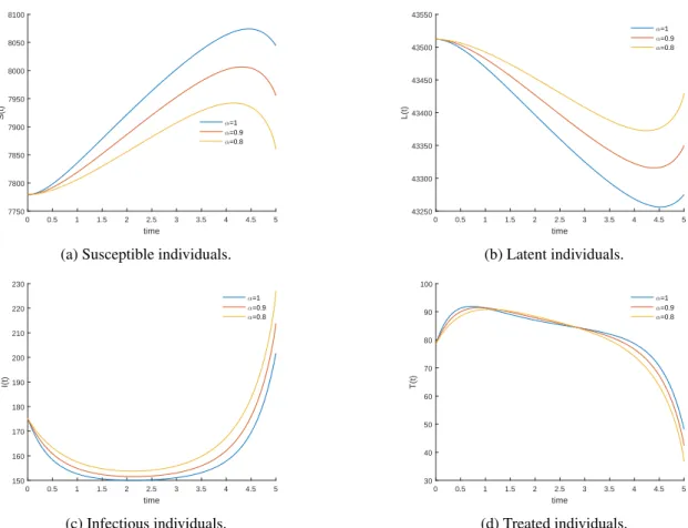
Without loss of generality, we considered the fractional order derivativesα = 1.0, 0.9and0.8. In Figures3and

4a, we find the solutions of the fractional optimal control problem for those values ofα. We can see that a change in the value ofα, corresponds significant variations of the state and control variables. The existence of an endemic situation (R0> 1), a very large initial number of latent individuals (about 84% of population), and a control that

vanishes at the end of the time interval motivates that, in the end of the time interval, the number of infected individuals exceeds its initial value. Beyond those values ofα, others values less than one were also tested, but the results do not change qualitatively. We note that, in all the experiments, decreasingαmeant increasing the number of infected, as Figure3cevidences.

In Figure4b, the efficacy function [15] is displayed. It is defined by

F (t) = I(0)− I

∗_(t)

I(0) = 1−

I∗(t)

I(0),

whereI∗(t)is the optimal solution associated with the fractional optimal control andI(0)is the corresponding initial condition. This function measures the proportional variation in the number of infectious individuals after the application of the controlu∗, by comparing the number of infected individuals at timetwith the initial valueI(0). We observe thatF (t)exhibits the inverse tendency ofI(t). OnceI(t)ends with values bigger than its initial value,

F (t)ends with negative values.

To assess the cost and the effectiveness of the proposed fractional control measure during the intervention period, some summary measures are presented. The total cases averted by the intervention, during the time periodtf, is

defined in [15] by

A = tfI(0)−

∫ tf

0

I∗(t) dt,

whereI∗(t)is the optimal solution associated with the fractional optimal controlu∗andI(0)is the corresponding initial condition. Note that this initial condition is obtained as the equilibrium proportionIof system (4) without treatment intervention, which is independent on time, so thattfI(0) =

∫ tf

0

I dt represents the total infectious cases over the given period oftf years. We define effectiveness as the proportion of cases averted on the total cases

possible under no intervention [15]:

F = A tfI(0) = 1− ∫ tf 0 I∗(t) dt tfI(0) .

The total cost associated with the intervention is defined in [15] by

T C =

∫ tf

0

time 0 0.5 1 1.5 2 2.5 3 3.5 4 4.5 5 S(t) 7750 7800 7850 7900 7950 8000 8050 8100 α=1 α=0.9 α=0.8

(a) Susceptible individuals.

time 0 0.5 1 1.5 2 2.5 3 3.5 4 4.5 5 L(t) 43250 43300 43350 43400 43450 43500 43550 α=1 α=0.9 α=0.8 (b) Latent individuals. time 0 0.5 1 1.5 2 2.5 3 3.5 4 4.5 5 I(t) 150 160 170 180 190 200 210 220 230 α=1 α=0.9 α=0.8 (c) Infectious individuals. time 0 0.5 1 1.5 2 2.5 3 3.5 4 4.5 5 T(t) 30 40 50 60 70 80 90 100 α=1 α=0.9 α=0.8 (d) Treated individuals.

Figure 3. State variables of the fractional optimal control problem (3)–(6), with values from Table1, weightB = 0.15, and

the fractional order derivativesα = 1.0, 0.9and0.8.

time 0 0.5 1 1.5 2 2.5 3 3.5 4 4.5 5 u(t) 0 0.1 0.2 0.3 0.4 0.5 0.6 0.7 0.8 0.9 1 α=1 α=0.9 α=0.8

(a) Optimal control, u.

time 0 0.5 1 1.5 2 2.5 3 3.5 4 4.5 5 F(t) -0.3 -0.25 -0.2 -0.15 -0.1 -0.05 0 0.05 0.1 0.15 α=1 α=0.9 α=0.8 (b) Efficacy functionF (t).

Figure 4. Control functionu(t)and efficacy functionF (t)associated to the fractional optimal control problem (3)–(6), with

values from Table1, weightB = 0.15, and the fractional order derivativesα = 1.0, 0.9and0.8.

whereCcorresponds to the unit cost, per person, of detection and treatment of infectious individuals. Following [11,15], the average cost-effectiveness ratio is given by

ACER = T C

In Table 4, the cost-effectiveness measures, for the fractional optimal control problem we have analysed, are summarized. These results show the effectiveness of the control to reduce TB infectious individuals and the superiority of the classical model (α = 1).

Table 4. Summary of cost-effectiveness measures for classical and fractional (0 < α < 1) TB disease optimal control

problems. Parameters according to Tables1and3withC = 1.

α A T C ACER F

1.0 88.6409 617.147 6.96233 0.101150

0.9 73.4419 608.801 8.28956 0.083806

0.80 54.8307 597.161 10.891 0.062568

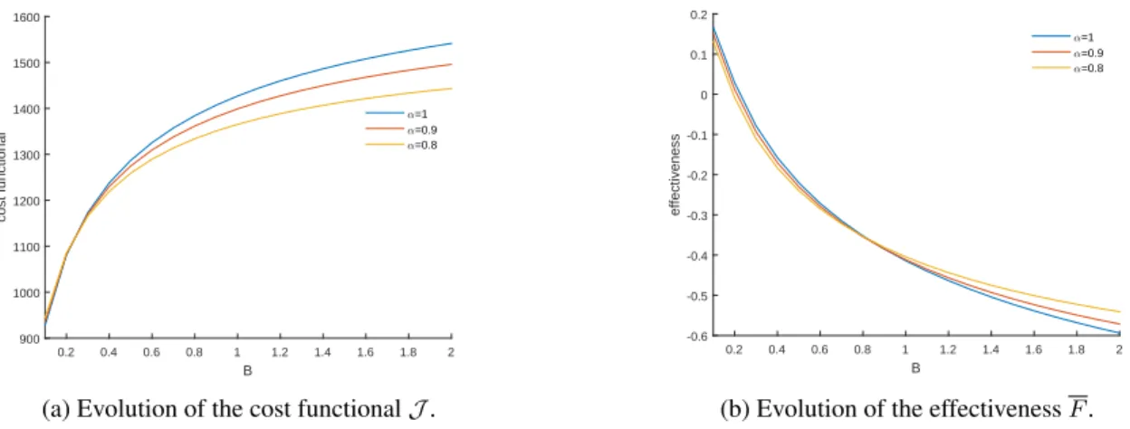
The impact of the variation of the weightBon the cost functional is displayed in Figure5a, and the effectiveness measureF is displayed in Figure5b. When the cost of treatment increases, we observe that the fractional model can be more effective in reducing the number of infective individuals at a not so high cost (Figure5a).

B 0.2 0.4 0.6 0.8 1 1.2 1.4 1.6 1.8 2 cost functional 900 1000 1100 1200 1300 1400 1500 1600 α=1 α=0.9 α=0.8

(a) Evolution of the cost functionalJ.

B 0.2 0.4 0.6 0.8 1 1.2 1.4 1.6 1.8 2 effectiveness -0.6 -0.5 -0.4 -0.3 -0.2 -0.1 0 0.1 0.2 α=1 α=0.9 α=0.8

(b) Evolution of the effectivenessF.

Figure 5. Impact of the variation of the weightBon the cost functional value,J, (left) and on the effectiveness measureF

(right) for fractional order derivativesα = 1.0,0.9and0.8.

4. Conclusions

A sensitivity analysis was carried out for the basic reproduction number of the TB model [24], proving that the most important parameter to have into account is the natural death rateµ. The application of optimal control to the fractional TB model shows that treatment is effective on the reduction of infected individuals. A change in the value of the fractional derivative order,α, corresponds to substantial variations on the solutions of the fractional optimal control problem. The fractional model (0 < α < 1) is recommended when treatment is expensive, and only in that case, because in that situation it is more effective and not so costly as the classical model.

Acknowledgements

Rosa was supported by the Portuguese Foundation for Science and Technology (FCT) through IT (project UID/EEA/50008/2019); Torres by FCT through CIDMA (project UID/MAT/04106/2019) and TOCCATA (project PTDC/EEI-AUT/2933/2014 funded by FEDER and COMPETE 2020).

REFERENCES

1. H. M. Ali, F. Lobo Pereira and S. M. A. Gama, A new approach to the Pontryagin maximum principle for nonlinear fractional optimal control problems, Math. Methods Appl. Sci. 39 (2016), no. 13, 3640–3649.

2. R. Almeida, S. Pooseh and D. F. M. Torres, Computational methods in the fractional calculus of variations, Imperial College Press, London, 2015.

3. N. Chitnis, J. M. Hyman and J. M. Cushing, Determining important parameters in the spread of malaria through the sensitivity analysis of a mathematical model, Bull. Math. Biol. 70 (2008), no. 5, 1272–1296.

4. A. Debbouche, J. J. Nieto and D. F. M. Torres, Optimal solutions to relaxation in multiple control problems of Sobolev type with nonlocal nonlinear fractional differential equations, J. Optim. Theory Appl. 174 (2017), no. 1, 7–31. arXiv:1504.05153 5. R. Denysiuk, C. J. Silva and D. F. M. Torres, Multiobjective approach to optimal control for a tuberculosis model, Optim. Methods

Softw. 30 (2015), no. 5, 893–910. arXiv:1412.0528

6. K. Diethelm, N. J. Ford, A. D. Freed and Yu. Luchko, Algorithms for the fractional calculus: a selection of numerical methods, Comput. Methods Appl. Mech. Engrg. 194 (2005), no. 6-8, 743–773.

7. S. Jahanshahi and D. F. M. Torres, A simple accurate method for solving fractional variational and optimal control problems, J. Optim. Theory Appl. 174 (2017), no. 1, 156–175. arXiv:1601.06416

8. R. Kamocki, Pontryagin maximum principle for fractional ordinary optimal control problems, Math. Methods Appl. Sci. 37 (2014), no. 11, 1668–1686.

9. A. B. Malinowska and D. F. M. Torres, Introduction to the fractional calculus of variations, Imperial College Press, London, 2012. 10. M. A. Mikucki, Sensitivity analysis of the basic reproduction number and other quantities for infectious disease models, PhD thesis,

Colorado State University, 2012.

11. K. O. Okosun, O. Rachid and N. Marcus, Optimal control strategies and cost-effectiveness analysis of a malaria model, Biosystems 111(2013), no. 2, 83–101.

12. I. Podlubny, Fractional differential equations, Mathematics in Science and Engineering, 198, Academic Press, Inc., San Diego, CA, 1999.

13. D. R. Powell, J. Fair, R. J. LeClaire, L. M. Moore and D. Thompson, Sensitivity analysis of an infectious disease model, Proc. Int. System Dynamics Conference, Boston, MA, 2005.

14. H. S. Rodrigues, M. T. T. Monteiro and D. F. M. Torres, Sensitivity analysis in a dengue epidemiological model, Conference Papers in Mathematics 2013 (2013), Art. ID 721406, 7 pp. arXiv:1307.0202

15. P. Rodrigues, C. J. Silva and D. F. M. Torres, Cost-effectiveness analysis of optimal control measures for tuberculosis, Bull. Math. Biol. 76 (2014), no. 10, 2627–2645. arXiv:1409.3496

16. M. R. Sidi Ammi, I. Jamiai and D. F. M. Torres, Global existence of solutions for a fractional Caputo nonlocal thermistor problem, Adv. Difference Equ. 2017 (2017), Paper no. 363, 14 pp. arXiv:1711.00143

17. C. J. Silva, H. Maurer and D. F. M. Torres, Optimal control of a tuberculosis model with state and control delays, Math. Biosci. Eng. 14(2017), no. 1, 321–337. arXiv:1606.08721

18. C. J. Silva and D. F. M. Torres, Optimal control strategies for tuberculosis treatment: a case study in Angola, Numer. Algebra Control Optim. 2 (2012), no. 3, 601–617. arXiv:1203.3255

19. C. J. Silva and D. F. M. Torres, Optimal control for a tuberculosis model with reinfection and post-exposure interventions, Math. Biosci. 244 (2013), no. 2, 154–164. arXiv:1305.2145

20. C. J. Silva and D. F. M. Torres, Optimal control of tuberculosis: a review, in Dynamics, games and science, 701–722, CIM Ser. Math. Sci., 1, Springer, Cham, 2015. arXiv:1406.3456

21. N. H. Sweilam and S. M. Al-Mekhlafi, Numerical study for multi-strain tuberculosis (TB) model of variable-order fractional derivatives, J. Adv. Res. 7 (2016), no. 2, 271–283.

22. P. van den Driessche, Reproduction numbers of infectious disease models, Infect. Disease Model. 2 (2017), no. 3, 288–303. 23. WHO, Global Tuberculosis Report 2016, World Health Organization, 2016.

24. W. Wojtak, C. J. Silva and D. F. M. Torres, Uniform asymptotic stability of a fractional tuberculosis model, Math. Model. Nat. Phenom. 13 (2018), no. 1, Art. 9, 10 pp. arXiv:1801.07059

25. Y. Yang, J. Li, Z. Ma and L. Liu, Global stability of two models with incomplete treatment for tuberculosis, Chaos Solitons Fractals 43(2010), no. 1-12, 79–85.