Short Wave Multipolar antenna for propagation by nviS effect
Igor Pereira a1, Maria João Martins a2, António Baptista b, Mariano Gonçalves c
a CINAMIL - Centro de Investigação da Academia Militar, Academia Militar, Lisboa, Portugal b Departamento de Engenharia Eletrotécnica, Instituto Superior Técnico, Lisboa, Portugal
c EID - Empresa de Investigação e Desenvolvimento de Eletrónica, Charneca da caparica, Portugal
ABSTRACT
The objectives of this papper is to design, build and test an antenna resonant at the frequencies of 4, 5, 6, and 7 MHz, in the high frequency band (HF). With this antenna we want to explore and use NVIS (Near Vertical Incidence Sky wave), which consists in using the ionosphere as a reflector layer of sky waves, that reach the ionosphere with angles near vertical incidence. When reflected, these waves achieve distances from dozens to hundreds of kilometers for the established communication. For short distances, this technique is useful to surpass obstacles, such as those caused by rugged terrain between the terminals of the connection. The theoretical design of this antenna, which is composed by four half-wave dipoles, each one resonant at one of the given frequencies, was made. The parameters of the antenna and the radiation diagrams were obtained by using an antenna simulation tool.
Since the ionsphere is used as a reflective layer of skywaves that arrive from the antenna, the propagation in the ionosphere was also studied. The antenna was then built and tested, and a good accordance between theoretical and experimental results was achieved.
Keywords: High frequency (HF), NVIS (Near Vertical Incidence Sky wave),
ionosphere, communication, half-wave dipoles.
RESUMO
Este artigo tem como objetivo o projeto e construção de uma antena resso-nante nas frequências de 4, 5, 6 e 7 MHz, ou seja, na banda da onda curta (HF). Com esta antena pretende-se explorar a utilização do conceito NVIS (Near Vertical Incidence Sky wave), que consiste na utilização da ionosfera
como meio refletor das ondas que ao chegarem à ionosfera, com ângulos perto da incidência vertical, são refletidas, atingindo-se distâncias que vão desde as dezenas de quilómetros até às centenas de quilómetros, para a comunicação estabelecida, dependendo do ângulo de emissão. Esta forma de transmissão é útil para curtas distâncias, pois permite ultrapassar obstáculos entre os terminais da ligação, tais como os devidos a orografia acentuada. Foi efetuado o dimensionamento teórico da antena, que é constituída por quatro dipolos de meia onda, cada um ressonante a uma das frequências anteriores. Obtiveram-se os diagramas de radiação e os parâmetros da an-tena recorrendo à utilização de uma ferramenta de simulação de anan-tenas. Estudou-se a propagação na ionosfera visto que esta é utilizada como ca-mada refletora das ondas provenientes da antena.
Posteriormente construiu-se a antena e ensaiou-se a mesma, obtendo-se um bom acordo entre os resultados teóricos e experimentais.
Palavras Chave: Onda curta (HF), NVIS (Near Vertical Incidence Sky
wave), ionosfera, comunicação, dipolos de meia onda.
1. INTRODUCTION
Short wave communications fell into disuse with the rise of sattelites, but have been emerging again particularly in military and emergency communications. Currently the Deployed National Forces (FNDs) have missions in theaters of operations (TO) with predominantly mountainous terrain and dense forest areas. These factors hinder the communications by ground wave or line of sight in the VHF and UHF bands. This difficulty is countered through the use of short wave communications, that use the ionoshpere as a reflective layer, achieving distances of thousands of kilometers, however in order to achieve these distances the emission antennas must use a maximum angle of 30º. When it is necessary to establish communications over distances from dozens to a couple hundreds of kilometers, we use antennas with high an-gles of elevation, near the vertical incidence at the ionosphere (70º to 90º). The simplicity of operation and mobility of the communication systems by NVIS effect is what makes this kind of communications the most suitable for a battle field, conflict area or places that have been subjected to an emergency situation and the permanent communications have been affected. Therefore and taking into account these paragraphs, it’s of high interest to stu-dy, develop and improve the actual means of communications by NVIS effect.
2. THEORETICAL DESIGN
In this chapter we will design the antenna prototype, wich is composed by four half-wave dipoles, and we will obtain the expressions for the radiated fields and the radiation diagrams by using Matlab and MMANA-GAL envi-ronments. But first we will study the behaviour of a single half-wave dipole.
2.1. the half-Wave Dipole
The half-wave dipole is one of the most usable linear antennas, it’s called that way because it’s physical length is equal to half of the wavelength (λ) at a given resonance frequency.
The radiated fields of a half-wave dipole are given by the following expressions: (1)
(2)
where the vacuum characteristic impedance is given by ,
IM is the maximum current in the dipole, is the air propagation
constant, r is the distance between the source and the point where we are evaluating the ratiated fields, and the angle θ is the colatitude.
So by analysing these expressions (1) and (2), we notice that for the
ra-diation zone the fields E and H are orthogonal and only have Eθ and Hφ
components (TEM mode).
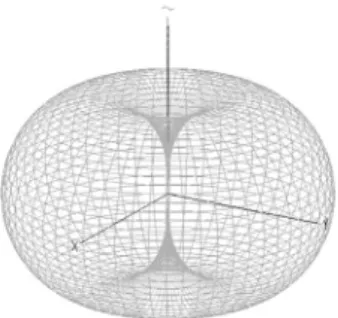
The three-dimensional radiation diagram for an half-wave dipole oriented in the z-axis is given in Figure 1.
Figure 1 - Three-dimensional radiation diagram
for an half-wave dipole oriented in the z-axis.
As we can see in Figure 1, an half-wave dipole has a three-dimensional radiation diagram with a shape of a “donut”, and has two kinds of points of interest: the zeros, that are coincident with the orientation of the dipole, and the maximums that are located perpendicular to the orientation of the dipole. These conditions are a determinant factor when choosing the orientation and polariza-tion of the antenna. If a dipole is placed vertically above the ground it will presente vertical polarization and the maximums in the horizontal. On the other hand if it is placed horizontally it will have horizontal polarization and the maximums vertically. Hence we pretend to explore communications by NVIS effect, the dipoles of the antenna will be defined horizontally so that the maximum of the radiation field will be directed to the ionosphere.
2.2. theoretical DeSign of the antenna
The antenna developed in this study has the following planar design given in Figure 2.
As it is seen in Figure 2, the antenna is composed by four half-wave dipoles with the following characteristics:
The first dipole (1) is oriented in the y-axis, it has a frequency f1=4 MHz, a corres-pondent wavelength λ1 = f1/c = 75 m, and a physical length of l1 = λ1/2 = 37,5 m; For the second dipole (2), which is oriented in the x-axis we have a frequency f2 = 5 MHz, a wavelenth of λ2 = f2/c = 60 m, and a physical length l2 = λ2/2 = 30 m; The third dipole (3) is oriented in the y’-axis and has a frequency f3 = 6 MHz, a wavelength λ3 = f3/c = 50 m, and physical length l3 = λ3/2 = 25 m;
The last, and fourth, dipole (4) is oriented in the x’-axis and has a frequency f4 = 7 MHz, wavelength λ4 = f4/c = 42,86 m, and a physical length of l4 = λ4/2 = 21,43 m. Now to calculate the electric fields for each dipole we use the expression (3): (3)
Now computing expression (3) for each dipole we obtain: (4) (5) (6) (7) where
At this point we have the radiated electric field for each dipole, now we need to “combine” them in order to get a valid expression for the all set of the antenna, in order to do that we do a vectorial sum:
And so as a final expression for the antenna we get:
(9)
We know that this expression, for the square of the modulus of the total electric field, is valid because it verifies the radiation condition, that means when r → ∞, the quantity
2.3. SiMulation of the DiagraM
The first simulation was made in Matlab environment. And in order to get results near to the reality, I computed the expression (9) introducing only one resonance frequency at a time. The generator feeds all the dipoles at the same time, however it only injects one frequency, so although all the dipoles are being fed, and have little contribuitions for the diagrams avoiding zeros, it is the dipole ressonante at that frequency that overruns the diagram. The diagrams obtained are shown in Figure 3.
Figure 3 – Radiation diagrams for the projected frequencies,
We notice that the results from Figure 3 are accurated because we hopped to see zeros in the orientation of each dipole, and that’s what happened. The second simulation was taken in the MMANA-GAL basic environment. And also here I did another approximation to reality, because it is not practical to elevate a planar antenna with this dimensions to an height of 4 meters above the ground. That is why it was adopted a configuration of inverted “v”, as we can see on Figure 4.
Figure 4 - Configuration of inverted “v”.
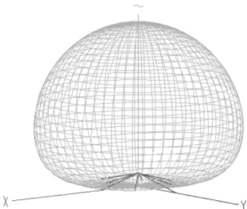
For this situation, Figure 4, the following three-dimensional diagram, Figure 5, was obtained using MMANA-GAL basic.
Figure 5 - Three-dimensional diagram for the projected
antenna.
It is possible to see that we only have one half of the diagram, which happens because now we are not in free space, and so due to the ground effect, the symmetric lobe is suppressed.
We can also see that this diagram fulfills the conditions that we want because it concentrates the energy in the z-axis direction, and so at the ionosphere direction.
3. IONOSPHERIC PROPAGATION
The ionosphere is a region from the upper atmosphere, which extends from an altitude of 60 to 600 kilometers. It is a zone composed by neutral mo-lecules sensitive to UV solar radiation, that ionizes these momo-lecules.
In this region the atmospheric pressure and air density are so low, the energy of the ions so high, and though the atraction force between positi-ve and negatipositi-ve charges still exists, the electrons can mopositi-ve freely during some time before they recombine. The existence of an high free electron density is what makes short waves to refract and eventually to reflect back to earth surface.
3.1. electron DenSity
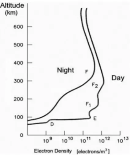
In the ionosphere there are two simultaneous processes happening, the formation of elctron-ion pairs by ionization of neutral molecules, and the recombination of the electron-ion pairs[5]. Though the density of positive ions is equal to the electron density, it is the electron density that matters to short wave communications because electrons have much lower mass than positive ions, and so electrons move faster and lead the processes. As it is expected the electron density isn’t the same for all the extension of the ionosphere, because this density is afected by temperature, preassure, air density, and the amount of solar radiation that reaches the earth. So it is also expected that the electron density is different during the day and night, and from summer to winter. In Figure 6 the evollution of the electron density with the altitude for day and night is shown.
3.2. layer MoDel
The ionosphere has a great extension in height, and as we know there are different conditions for different heights. So based on Figure 6, we can consider some layers with different mean electron density.
The first considered layer is the D layer that exists between 60 and 90 km. The next layer is the E layer and its height is comprehended between 90
and 140 km. During the day there are two more layers the F1 between 140
and 200 km, and F2 from 200 to 500 km. However during nightime the
D and E layers disapear and the F1 and F2 combine and form the F layer.
3.3. plaSMa frequency
The plasma frequency fp is a very important parameter, because it is the
threshold between a reflected wave or a propageted wave.
When a radio wave with a certain frequency f, enters a plasma, if the plasma
frequency is lower than the frequency of the wave, f > fp, that wave
propa-gates through the plasma. On the other hand if fp > f the wave is reflected. The plasma frequency is given by the following expression:
(10)
where q = -1,59*10-19 C is the charge of an electron, N
e [electrons.m-3] is
the electron density, me = 9.107 x 10⁻³¹ Kg is the mass os an electron and is the electric permittivity of the air.
On Table 1 we can see the plasma frequency for each layer, these values were calculated considering the values of Figure 6 for the electron densities.
3.4. chapMan’S MoDel
As seen before the electron densities varies within the ionosphere for many reasons, that had been mentioned before on section 3.1.
Sidney Chapman was the first to establish a mathematical model for the evolution of the electron densities as a fuction of height in 1927.
The expression he developped is the following one:
(11)
where Nm is the maximum electronic density, hm the height in kilometers
(km) where Nm is verified, h is the height in km where it is wanted to
cal-culate the electron density, χ is the angle that the Sun does with the earth’s vertical and H is a scale height in km, given by:
(12)
where kB = 1,38*10-23 [J°K-1] is the Boltzman constant, T is the absolute
temperature in Kelvin degrees (°K), m is the average molecular mass and g = 9,8 [m/s2] is the gravitational acceleration.
In Figure 7 it is shown the curve for the Chapman’s model is presented:
4. CONSTRUCTION AND RESULTS 4.1. builDing
The construction of the prototype of antenna was made at the Military Academy laboratory, and it can be summurized into three steps:
The first one is the connection of the inner contacts within a PVC tube in order to get protection and robustness. As can be seen in Figure 8.
Figure 8 - Central module of the prototype.
Notice that half of the plugs (female plugs) are red and the other half are black, so we can have a positive side (+) and a negative one (-).
The following step was to cut and attach the male plugs into the wire that compose a dipole. In Figure 9 can be seen the four dipoles built.
50 Ω. This differance of impedances may cause problems when transfering power from the generator to the antenna, so its necessary to create a balanced line between the ressonant circuit and the line that feeds the circuit.
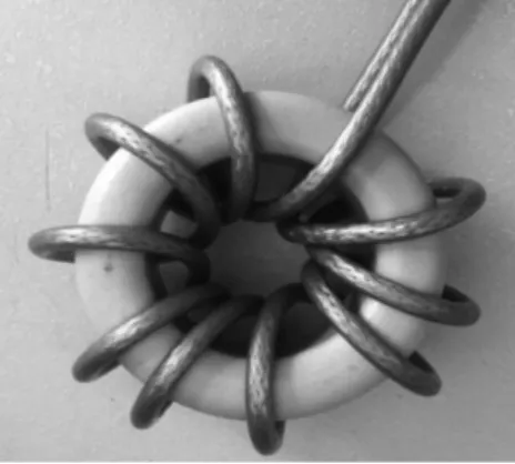
To build the balun we used a toroidal ferrite core and a thin coaxial cable, which did nine turns arround the toroidal core, as can be seen in Figure 10.
Figure 10 – Balun with nine
The balun was then connected into the central module and the antenna prototype is ready to be assembled.
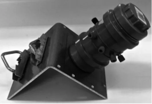
In Figure 11 is shown the antenna fully assembled in the day of the tests.
4.2. reSultS
To measure the results of the antenna a Network Analizer was used. In this device’s display it is possible to see the response of the antenna.
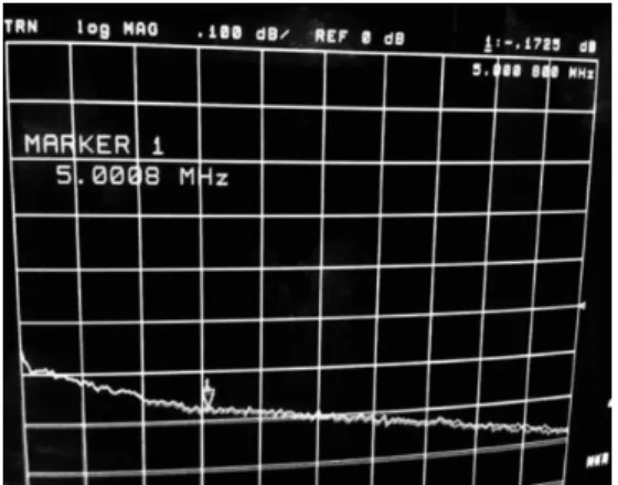
The first measures were made to characterize the insertion loss of the ba-lun, and in Figure 12 the curve obatined in the network analizer is shown. Figure 12 shows de insertion loss caused by the balun at 5 MHz and the value is on the upper right-hand side. Since the curve is the same for the remaining frequencies, the figures will not be shown but the results are presented in Table 2.
Table 2 - Insertion loss values.
As we can see adding the balun to the circuit of the antenna do not cause remarkable losses.
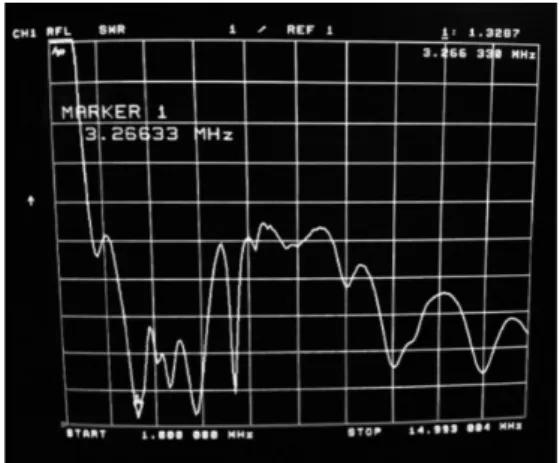
Now the parameters of the antenna, namely the Standing Wave Ratio (SWR), (on Figure 13), and the return loss (on Figure 14) are measured.
Regarding to the SWR the minimums present in the curve in the display (Figure 13), must occur at the resonance frequencies of the antenna. In the following Figure 13, the resonance frequency, given by the marker, and the value of the SWR on the upper right-hand side are shown.
Figure 13 – SWR at the first resonance frequency.
Only shown the figure for the first resonance frequency is presented, because the curve of the SWR is stationary. So the readings for the other resonance frequencies are given on Table 3.
Table 3 – Values of the measurements for the SWR.
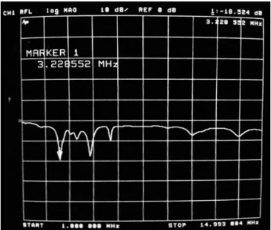
In Figure 14, the value for the return loss corresponding to the first reso-nance frequencyis shown.
The reading process is the same as the one used in Figure 13, the marker gives the resonance frequency, and the value of the return loss can be seen in the upper right-hand side.
Figure 14 - Return loss at the first resonance frequency.
For the remaining resonance frequencies the values of return loss can be seen in Table 4.
Table 4 - Values of the measurements for the return loss.
After analyzing tables 3 and 4, it is possible to notice that the values of the resonance frequencies dropped about 800 kHz from the projected ones, (4, 5, 6 and 7 MHz). This situation may have several causes because the designed
frequencies is the geometry, beacause when setting-up the antenna, and due to terrain irregularities, the dipoles were not perfectly separated from each other. Besides these effects, the values for the SWR and return loss, are satisfa-tory because they are in the range of acceptable values for these antennas.
5. CONCLUSIONS
An antenna prototype for NVIS communication was designed which is composed by four half-wave dipoles. A theoretical study of this antenna was performed and the radiated fields expressions and both two and three--dimensions radiation diagrams were obtained.
Then the antenna was designed and the diagrams obtained using Matlab and MMANA-GAL basic were agreed with the theoretical results.
After all this calculations and simulations it was studied the crucial issue for NVIS communications, the ionosphere. The plasma frequency is the parameter that determines if the wave propagates or reflects to earth. The results obtained from the mean values of the electron density in each layer are presented in Table 1. The last part of this work was the construction and tests of the prototype. The measurements performed for the SWR and return loss, were made in a network analizer, and they were very satisfatory because all of them were in the range of the aceptable values.
This prototype antenna is a very valuable asset for the Portuguese Army, which is envolved in many international missions where the terrain is hi-ghly mountainous and irregular, and therefore it is not possible to get a communication link via satellite or by ground wave.
BIBLIOGRAPHICAL REFERENCES
BALANIS, C. A. (2005). Antenna Theory: Analyssis and Design, John Wiley & Sons Inc.
MARTINS, Maria J. (2002). Propagação e Radiação de Ondas Electromagnéticas – Radiação, Academia Militar, Lisboa.
FARO, M. de A. (1980). Propagação e Radiação de Ondas Electromagnéticas 2 – Radiação, Técnica A.E.I.S.T., Lisboa.
FIGANIER, J. (2002). Aspectos de Propagação na Atmosfera, Secção de Folhas IST.
CARR, J. J. (2001). Practical Antenna Handbook, MacGraw-Hill.
GREENMAN, M. (1999-2009). An Introduction to HF propagation and the Ionosphere. Internet: http://www.qsl.net/zl1bpu/IONO/iono101.htm, consultado em [18-Jul-2014].
POOLE, I. (1999). Radio Waves and the Ionosphere, QST ARRL.
Igor Pereira is a Lieutenant from the Signal Corps of Portuguese Army. He holds a Master degree in Military Electrical Engineering from the Portuguese Military Academy.
Maria João Martins Completed the ”Licenciatura” and Doctoral Degree, both at Instituto Superior Tecnico, Lisbon, where she taught as Professor in the Department of Electrical and Computer Engineering. She was an invited Professor in the Universities of Karlsruhe, Germany, (1992) and Rennes I, France (2004), She served as Expert-evaluator for the European Commission, in the 5th and 6th Framework Programs. She is since 2012 Professor in the Military Academy in Lisbon.
António Baptista Completed the ”Licenciatura”, Master and Doctoral Degree, at Instituto Superior Tecnico, Lisbon, where he has been teaching as Professor in the Department of Electrical and Computer Engineering to the present day. Mariano Gonçalves has a degree in Electrical and Computer Engineering. Currently he is Project Director with the EID - Empresa de Investigação e Desenvolvimento de Eletrónica.