Abstract— The study presented in this article is dedicated to the
backfire disk-on-rod antennas fed by a dipole or crossed dipole. For short, these are herein called backfire antennas. Backfire antenna constructions with different configurations of the big reflector are considered. The influence of the feed location in the backfire antenna construction upon the antenna characteristics is also examined. The studies were carried out with a corrugated-rod (disks attached to a metal rod) surface-wave structure. The results obtained may be applied to other types of surface-wave structures, such as dipole array, dielectric rod or dielectric-covered metal rod. The lengths of the investigated antennas ranged between 2λ and 4λ. The design carried out in these investigations may be used for creation of high efficiency backfire antennas.
Index Terms— backfire antenna, end-fire antenna, long backfire antenna, surface wave, surface-wave antenna, surface-wave structure.
I. INTRODUCTION
The backfire antenna is created by H. W. Ehrenspeck and his associates at the Air Force
Cambridge Research Center, Bedford, Mass. in 1959 [1]-[5]. It was obtained by placing of a big
reflector at the open end of an end-fire antenna perpendicularly to its axis. Thus, the antenna increases
its length for the surface wave which leads to the improvement of the antenna gain and directivity.
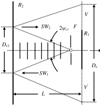
The geometry of the backfire antenna is shown in Fig. 1. It consists of a source F (for example, a
dipole or crossed dipole), a surface-wave structure S (dipole array, corrugated rod, dielectric rod or
dielectric-covered metal rod) and two parallel disk reflectors: small reflector R1 and big reflector R2.
In the figure, the antenna length is the distance between the reflectors R1 and R2, denoted by L. The
radiation mechanism of the backfire antenna is described in many references [4]-[10]. The first,
simplified model of the backfire antenna radiation mechanism was very rough approximation to the
real physical process in the antenna. It presents the backfire antenna as an end-fire antenna of
effective length Le equal to double the physical length L, or Le = 2L. The spherical wave radiated from
the source F is transformed in a surface wave SW1 by the surface-wave structure S. It terminates by
the big reflector R2, which reflects the surface wave SW2 toward the small reflector R1, where it is
radiated from the antenna aperture VV’ into the space. Thus, the radiation of the antenna is directed in
inverse direction in comparison with the radiation of the ordinary end-fire antenna used as a backfire
antenna prototype. Because of this reason it is called backfire antenna (antenne à rayonnement
inverse, антенна обратного излучения, еtc…). According to this model the directivity increase of
Study of Backfire Antennas
G. S. Kirov*, H. D. Hristov**
*
Department of Radio Engineering, Technical Uniersity of Varna, Studentska Str.1, 9010 Varna, Bulgaria e-mail: [email protected]the backfire antenna in comparison with the end-fire antenna should be 4 times (or 6 dB): 3 dB due to
the length of the antenna Le = 2L (the directivity of the relatively short surface-wave antenna is
proportional to its length) and 3 dB due to the presence of the big reflector which assures a radiation
from the antenna in only one hemisphere.
Fig. 1. The geometry of a backfire antenna.
It is found in practice that a bigger directivity increase (6 times or approximately 8 dB) may be
obtained by the backfire antenna using a phase corrected big reflector and accurate tuning of the
surface-wave structure. This result may be explained only by means of more rigorous model of the
backfire antenna radiation mechanism. Consistent with this model the surface wave is reflected
multiple times between the reflectors R1 and R2 of the semitransparent open cavity R1R2 before be
radiated from the virtual antenna aperture VV’. The diffraction effects on the both reflectors and the
direct radiation from the feed dipole should be also taken into account [7]-[10]. Our experiments with
backfire antennas have shown that Le equal to 6L gives the best result in regard to the optimum value
of the phase velocity of the surface wave. This model corresponds to six forward and backward
travels of the surface wave along the surface-wave structure or to a triple wave reflection from the big
reflector.
Because of its uncontestable advantages (simple and compact construction, reduced length and
good radiation performance) the backfire antennas have been widely used in various wireless
systems, mostly military, earth and spacecraft. Now they may be used for long-range point-to-point
applications, say WLAN, WISP and satellite links and in those cases where a gain between 15 dB and
25 dB and a bandwidth less than 10 % are required.
II. OPTIMUM PHASE VELOCITY AND DIMENSIONS OF THE BACKFIRE ANTENNA
In order to obtain maximum directivity and efficiency from the backfire antenna the phase velocity
R
2V
V
’L
R
1F
D
e1D
e2
ψ
crSW
1of the surface wave and the dimensions of the antenna should have optimum values.
A. Phase velocity
According to the Hansen-Woodyard condition [11], [12] the optimum value of the phase velocity
delay factor of an uniformly illuminated end-fire antenna is
c/v = 1 + λ0/(2L), L > 20λ0, (1)
where c is the free-space wave velocity, v is the phase velocity of the surface wave, and λ0
corresponds to f0 – the design (central or resonant) frequency.
The directivity of the end-fire antenna above an isotropic radiator in these conditions is
D = 7L/λ0 (2)
If the design is based on the optimum phase velocity and taper dimensions of the surface-wave
structure (non-uniformly illumination) the expressions (1) and (2) become
c/v = 1 + λ0/(qL), (3)
D = 10L/λ0, 3λ0 < L < 8λ0, (4)
where the coefficient q starts near 6 for L = λ0 and diminishes to approximately 3 for L between 3λ0
and 8λ0 and to 2 at 20λ0. The formulas (3) and (4) proposed by Ehrenspeck and Poehler [12], [13] are
based on the experimental investigations on Yagi-Uda antennas.
According to the Hansen-Woodyard condition and based on the simplified model of the backfire
antenna radiation mechanism [4], [6], [14] the optimum value of the phase velocity delay factor and
the directivity are given by
c/v = 1 + 0.234(λ0/L), L > 10λ0, (5)
D = 28L/λ0 (6)
The change of the phase velocity delay factor c/v as a function of the backfire antenna length in
wavelengths L/λ0 is shown in Fig. 2(a) with a dotted line. Better results can be obtained using
Ehrenspeck and Poehler experimental results [4]:
c/v = 1 + λ0/(2qL), (7)
D = 40L/λ0, 1.5λ0 < L < 4λ0 (8)
The variation of the phase velocity delay factor c/v consistent with the expression (7) is presented
in above figure with a dashed line. Finally, consistent with the model of the backfire antenna radiation
mechanism proposed herein (Le = 3L) the optimum value of c/v (Fig. 2(a),solid line) and the
directivity can be defined as follows
c/v = 1 + 0.078λ0/L, (9)
1.5 2 2.5 3 3.5 4 4.5 1
1.02 1.04 1.06 1.08 1.1 1.12 1.14 1.16
Length in wavelengths Ln
V
el
o
ci
ty
d
el
ay
f
ac
to
r
c/
v
(a)
2 2.5 3 3.5 4
1 1.02 1.04 1.06 1.08 1.1
Length in wavelengths Ln
V
el
o
ci
ty
d
el
ay
f
ac
to
r
c/
v
(b)
Fig. 2. Phase velocity delay factor versus backfire antenna length in wavelengths Ln = L/λ0: (a) different models of radiation
mechanism: solid line: Hristov and Kirov model – eq. (9); dashed line: Ehrenspeck and Poehler experimental values –
eq. (7); dotted line: Hansen – Woodyard condition – eq. (5); (b) comparison between theory and measurements: solid
line: Hristov and Kirov model – eq. (9); dashed line: Strom experimental values [5]; dotted line: Hristov and Kirov
experimental values.
In order to verify the validity of the proposed model of radiation mechanism the both curves of the phase velocity delay factor, the solid line according to the proposed model and the dashed line
consistent with the experimental results obtained by Strom [5] are presented in Fig. 2(b). In the same
figure our experimental results for two types of backfire antennas: an antenna with a feed near the big
reflector (dashed line coinciding with the Strom’s results) and an antenna with a feed near the small
reflector (dotted line) are also shown. A good agreement between the proposed model and the
measurement is found.
B. Feed location
The feed located between the two reflectors acts directly on the backfire antenna characteristics.
There are only two feed locations which assure normal work of the antenna. In the first manner of
feed the feed dipole F is located near the small reflector R1. The backfire antenna with this feed
location is preferable in the practice because of its good radiation characteristics. In the second
manner of feed the feed dipole F is located near the big reflector R2. The use of the backfire antenna
with this feed location is limited because of its lower gain (with 3-4 dB) compared to the antenna with
the first feed location. In the both cases the distance between the feed point and respective reflector is
λ0/4. Other points of feed location along the length of the backfire antenna are not suitable and are not
recommended [10].
C. Big reflector
The diameter of the big reflector R2 is related to the quantity of the reflected energy and to the
SW1 with phase velocity v and a spherical wave with velocity c. In the plane of the big reflector, in the
limits of so-called critical angle 2ψcr (or 2ψ < 2ψcr), the wave has a quasi-plane phase front and
effective radiation aperture of diameter De1 (Fig. 1):
De1 = 2Ltanψcr, (11)
where
tanψcr = ( / ) 1
2 −
v
c (12)
Having in mind (5) and (12) the diameter De1 is defined as a function of L/λ0 as follows
De1 =
1
.
4
L
/
λ
0 (13)The value 2ψcr divides the big reflector R2 into two regions. In the first region with 2ψ < 2ψcr the surface wave is predominant, while in the second one with 2ψ > 2ψcr the spherical wave plays
essential role in the wave distribution. Thus, the minimum diameter D2 of the backfire antenna big
reflector R2 should be equal to the constant-phase effective aperture, or D2 = De1. If the diameter D2
increases (the second region with 2ψ > 2ψcr) the phase front becomes spherical and a quadratic phase
distortion on the big reflector plane occurs. In the case where a tolerable phase distortion of π/2 rad at
the disk edge is assumed, the dimension of its diameter is given by [4]
D2 =
2
λ
0L
/
λ
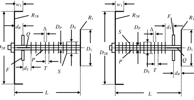
0 (14)Fig. 3. Some possible configurations of the big reflector: (a) disk reflector R2, (b) rimmed disk reflector R2R, (c) rimmed
reflector with step correction R2S, and (d) rimmed reflector with conical correction R2C.
Some possible configurations of the big reflector are shown in Fig. 3. Fig. 3(a) shows a plane
circular reflector R2. Its diameter D2 is defined by the expression (14). A rimmed disk reflector R2R of
(c)
(d)
D
2CD
20w
2w
1R
2CD
2(a)
(b)
R
2D
2Rw
1R
2RD
2SD
20w
1w
2diameter D2R is shown in Fig. 3(b). The rim decreases the levels of the backlobe and sidelobes and leads to an improvement of the antenna gain and directivity. The diameter D2R is calculated by the expression (14) and the rim width w1 is equal to a quarter-wave length
w1 = 0.25λ0 (15)
Further increase of the antenna directivity and efficiency can be obtained using a phase correction
in big reflector R2. Thus, the reflected wave will involve and the energy of the peripheral spherical
waves with a minimum phase shift [4],[10]. In this manner the ideal big reflector should consist of
two parts: a first plane part and a second parabolic one. In practice because of technological reasons
the simplified stepped and conically corrected big reflectors are mostly used. Fig. 3(c) shows a
rimmed stepped-corrected disk reflector R2S of diameter D2S with a inner diameter D20 and step width
w2. A rimmed conically-corrected disk reflector R2C of diameter D2C is shown in Fig. 3(d). The corresponding dimensions of the reflectors R2S and R2C are given by the expressions [4],[10]
D20 = (1.9 ÷ 2.0)λ0
L
/
λ
0 , (16)D2S = D2C = (2.9 ÷ 3.0)λ0
L
/
λ
0 , (17)w1 = w2 = 0.25λ0, (18)
which are in good agreement with the results of the experimental studies.
D. Length of the antenna
The backfire antenna can be considered as a parallel-plane resonator antenna with a standing
surface-wave field excited inside. In the virtual antenna aperture VV’ (Fig. 1) two basic phenomena
take place: multiple partial reflections from the small reflector R1 and multiple intensive radiations
from the open aperture area. The length of such radiating cavity must satisfy equation
L = n λS0/2 + L, for n = 1,2,3,…, (19)
where λS0 = v/f0 is the surface wave wavelength, L is the length correction due to the radiation, and n
is a real integer called standing-wave number. The experimental results show that
L = n(λ0/2), (20)
where n have the same integral values as in (19).
On the other hand, the antenna length depends directly on the required directivity (gain). It can be
approximately calculated by the expression
L≈ (D/A)λ0, (21)
where the values of the coefficient A are given in a Table I.
The accurate length of the backfire antenna can be defined by the mutual solution of equations
TABLE I.THE VALUES OF THE COEFFICIENT A FOR A BACKFIRE ANTENNA,L=2Λ0 TO 4Λ0
Type of the big reflector Coefficient A
R2R, a feed near the big reflector 20 - 25
R2R, a feed near the small reflector 40 - 50
R2C, a feed near the small reflector 60
The most often used in practice are the backfire antennas with lengths between 2λ0 and 6λ0. If a
higher directivity is required an use of backfire antenna arrays is recommended.
E. Small reflector
The dimension of the small reflector R1 acts essentially on the amplitude and phase field
distribution in the antenna aperture. In addition it is related to the feed efficiency in the case where the
feed is set near the small reflector. The very small values of this reflector transform the backfire
antenna into an ordinary end-fire antenna and decrease the directivity. On the other hand the high
values of the small reflector diameter close to the big reflector diameter also decrease the antenna
directivity because of a reduction of the aperture area (the antenna transforms in a high quality-factor
resonator).
The optimum value of the small reflector diameter increases with an increase of the antenna length
and can be found by [10]
D1 = (0.25 ÷ 0.45)λ0
L
/
λ
0 (22)The experimental studies show that for a backfire antenna with a length between 2λ0 and 6λ0 the
optimum value of the small reflector diameter ranges between 0.35λ and 1.1λ0.
III. DESIGN PROCEDURE FOR BACKFIRE ANTENNAS
There are only a few references dedicated to the backfire antennas design [4],[10]. It is not
considered even in some recently published books on an antenna design [12],[15]-[17]. A design
procedure for backfire antennas with circular reflectors and a corrugated-rod surface-wave structure,
fed by a dipole, is described here. It is based on studies in [10], and some new results obtained by the
authors. The results presented here may be applied to other types of surface-wave structures, such as
dipole array, dielectric rod, or dielectric-covered metal rod. The lengths of the antennas studied
ranged between 2λ0 and 4λ0, which are the most-used lengths, in practice. However, the range of the
proposed design may be extended by a simple extrapolation in the range of the antenna lengths from
2λ0 to 6λ0.
Three constructions of backfire antennas are considered in this design:
Fig. 4. A backfire antenna fed by a dipole located near the big reflector R2R (Antenna A1).
Fig. 5. A backfire antenna fed by a dipole set near the small reflector with a big reflector R2R (Antenna
A2).
- a backfire antenna fed by a dipole located near the small reflector with a big reflector R2C, an antenna A3 (Fig. 6).
Fig. 6. A backfire antenna fed by a dipole located near the small reflector with a big reflectorR2C
(Antenna A3).
Fig. 7. The practical implementation of a backfire antenna A3, L = 4 λ0.
The antenna A1 has the most simple construction but its gain is the lowest while the antenna A3 provides the highest gain with relatively more complex construction. The new antenna elements and dimensions in Fig. 4 – Fig. 6are denoted as follows: P is a metal rod (a rigid feed coaxial line), Q – a half-wavelength slot balun used to feed the symmetrical dipole by the coaxial line, D1 – a small
reflector diameter, DP – a metal rod diameter, DS – a disks diameter, dS and dR – distances between the dipole and the surface-wave structure, and the nearer reflector, respectively, T – a period of the surface-wave structure, and – a disks thickness.
D
2RL
D
1w
1R
2RR
1
d
Rd
SD
PD
ST
F
P
S
Q
D
2RL
D
1w
1R
2RR
1
D
PD
Sd
Sd
RS
P
F
T
Q
D
2CL
D
1w
1R
2CR
1D
PD
ST
d
Sd
RS
P
F
w
2The directivity, D, the central frequency of the antenna’s bandwidth, f0, and the type of the
surface-wave structure, S, are assumed known in this design. The design goal is to determine the basic
dimensions of the backfire antenna. The design procedure involves the following steps:
A. Length of the backfire antenna
The approximate length of the antenna is defined by the required directivity
0
10 ] [
10
λ
A
L
dB D
=
(23)using the Table I for the values of the coefficient A.
The final length of the antenna is defined according to the requirements of (20) and (21).
B. Optimum phase velocity of the backfire antenna
The optimum value of the phase velocity delay factor c/v is calculated by the expression (9). For
backfire antennas with lengths between 2λ0 and 4λ0 more accurate values obtained experimentally by the authors are given in Table II.
TABLE II.THE OPTIMUM VALUES OF THE PHASE VELOCITY DELAY FACTOR C/V FOR A BACKFIRE ANTENNA FOR L=2Λ0 TO 4Λ0
Type of the backfire antenna Phase velocity delay factor c/v
Antenna 1 (Fig. 4)
L = 2λ0
L = 3λ0
L = 4λ0
1.05 1.03 1.02
Antenna 2 (Fig. 5) 1.02
Antenna 3 (Fig. 6) 1.02
C. Dimensions of the big reflector
The diameter D2R for the backfire antennas A1 and A2 is defined by formula (14) and the rim width w1 is given by (15).
The diameter of the plane part of the big reflector D20 for the backfire antenna A3 is calculated by
(16) and the big reflector diameter D2C is given by (17). The rim width w1 and the step width w2 are
defined by (18).
D. Diameter of the small reflector
The optimum values of the small reflector diameter (obtained experimentally by the authors) are
given in Table III.
TABLE III.THE DIAMETER OF THE SMALL REFLECTOR OF A BACKFIRE ANTENNA, FOR L=2Λ0 TO 4Λ0
Type of the backfire antenna Diameter D1
Antenna 1 (Fig. 4) 0.295D2R
Antenna 2 (Fig. 5) 0.170D2R
Antenna 3 (Fig. 6) 0.150D2C
E. Distances from the dipole to the surface-wave structure, and the respective reflector
dS = dR = 0.25λ0 (24)
F. Surface-wave structure
Based on the optimum value of the ratio c/v found above the surface-wave structure dimensions DS,
DP, T and may be defined using the well known design procedure described in [18] or [16]. In the
case where a dielectric rod is used as a surface-wave structure the design procedure should be
accomplished consistent with the methods described for example in [16] or [12], [17].
G. Feed dipole
The design of the half-wavelength dipole (or crossed dipole) is classic and may be found in many
references[12],[15]-[17].
IV. PRACTICAL EXAMPLES
In order to verify the validity of the proposed design procedure, three backfire antennas were
desi-gned, fabricated and tested. A photograph of a backfire antenna with a corrugated-rod surface-wave
structure fed by a dipole set near the small reflector with a big reflector R2C and length L = 4λ0, λ0 =
13.6 cm, is shown in Fig. 7. This antenna construction (an antenna A3) was chosen as a basic antenna
configuration because of its high performance characteristics.
90 60 30 0 30 60 90
40 30 20 10 0
Angle (Degrees)
R
ad
ia
ti
o
n
P
at
te
rn
(
d
B
)
90 60 30 0 30 60 90
40 30 20 10 0
Angle (Degrees)
R
ad
ia
ti
o
n
P
at
te
rn
(
d
B
)
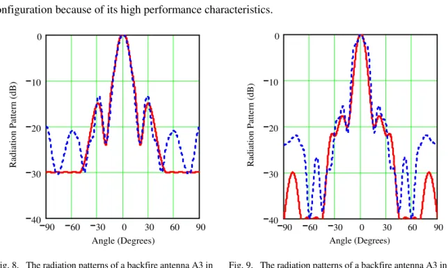
Fig. 8. The radiation patterns of a backfire antenna A3 in E–plane (solid line) and H-plane (dashed line):
L = 2 λ0, f = 2.2 GHz.
Fig. 9. The radiation patterns of a backfire antenna A3 in E–plane (solid line) and H-plane (dashed line):
L = 3 λ0, f = 2.25 GHz.
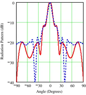
The radiation patterns in E- (solid line) and H-plane (dashed line) of the fabricated antennas with
lengths L = 2λ0, 3λ0, and 4λ0 were measured and shown in Fig. 8 – Fig. 10, respectively. The
directivities of the antennas were defined by an integration of their radiation patterns and the results
obtained are illustrated in Fig. 11 for lengths L = 2λ0, f0 = 2.2 GHz (dotted line), L = 3λ0, f0 = 2.25
GHz (dashed line), and L = 4λ0, f0 = 2.2 GHz (solid line). Fig. 12 illustrates the input match
VSWR is 12 % and for a 1.5:1 VSWR is 8.6 %, respectively. The influence of the antenna length on
the bandwidth is insignificant.
Fig. 10. The radiation patterns of a backfire antenna A3 in E–plane (solid line) and H-plane (dashed line): L = 4 λ0,
f = 2.2 GHz.
2.15 2.2 2.25 2.3 2.35 2.4 15 17 19 21 23 25 Frequency (GHz) D ir ec ti v it y ( d B )
2 2.05 2.1 2.15 2.2 2.25 2.3 2.35 1 1.25 1.5 1.75 2 2.25 2.5 Frequency (GHz) V o lt ag e st an d in g -w av e ra ti o V S W R
Fig. 11. The directivities of three backfire antennas A3 with lengths L = 2 λ0 (dotted line), L = 3 λ0 (dashed line),
and L = 4 λ0 solid line).
Fig. 12. Measured VSWR as function of frequency for a backfire antenna A3 with length L = 4 λ0.
The dimensions of the backfire antennas designed according to the above described design
procedure are summarized in Table IV. In the last row of the table the measured and theoretical
directivity, calculated by means of (10),Dm,are shown for comparison. Good agreement between the
designed, measured and theoretical values was found. The results obtained showed that the proposed
design procedure can be used for creation of high efficiency microwave communication antennas.
90 60 30 0 30 60 90
TABLE IV.RESULTS OBTAINED FOR THREE BACKFIRE ANTENNAS,L=2Λ0,3Λ0, AND 4Λ0
Antenna parameter (Dimension) Example 1 Example 2 Example 3
Design directivity D 21 dB 22.2 dB 24 dB
Design frequency f0 2.2 GHz 2.25 GHz 2.2 GHz
Approximate length of the antenna La 2.10 λ0 2.77 λ0 4.19 λ0
Final length of the backfire antenna L 272.7 mm (2 λ0) 400.0 mm (3 λ0) 545.4 mm (4 λ0)
Optimum phase velocity delay factor c/v 1.02 1.02 1.02
Inner diameter D20 366.4 mm (2.687 λ0) 438.8 mm (3.291 λ0) 518.2 mm (3.800 λ0)
Diameter of the big reflector D2C 559.2 mm (4.101 λ0) 669.7 mm (5.023 λ0) 790.9 mm (5.800 λ0)
Rim width w1 34.1 mm (0.25 λ0) 33.3 mm (0.25 λ0) 34.1 mm (0.25 λ0)
Step width w2 34.1 mm (0.25 λ0) 33.3 mm (0.25 λ0) 34.1 mm (0.25 λ0)
Diameter of the small reflector D1 83.9 mm (0.615λ0) 100.4 mm (0.753λ0) 118.6 mm (0.870λ0)
Distances dS, dR 34.1 mm (0.25 λ0) 33.3 mm (0.25 λ0) 34.1 mm (0.25 λ0)
Measured (and theoretical) directivity Dm 20.9 dB (20.8 dB) 22.1 dB (22.5 dB) 23.8 dB (23.8 dB)
ACKNOWLEDGMENT
The authors wish to acknowledge the financial support under the Chilean Anillos Bicentenario
Project ACT-53/2010-2012.
REFERENCES
[1] H.W. Ehrenspeck, Reflection antenna employing multiple director elements and multiple reflection of energy to effect
increased gain, US Patent No. 3,122,745, Febr. 1964, (Filed May 1959).
[2] H.W. Ehrenspeck, “The backfire antenna, a new type of directional line source”, Proc. IRE, vol. 48, No. 1, pp. 109-
110, 1960.
[3] H.W. Ehrenspeck,, “The backfire antenna: new results”. Proc. IEEE, vol. 53, No. 6, pp. 639-641, 1965.
[4] F.J. Zucker, “The backfire antenna: a qualitative approach to its design”, Proc. IEEE, vol. 53, No. 7, pp. 746-747,
1965.
[5] J.A. Strom, A dielectric-rod backfire antenna, AFCRL Report 69-0347, August 1969.
[6] H.D. Hristov, Study of backfire antennas with surface-wave structures, Ph.D. Thesis, Sofia, 1973 (In Bulgarian).
[7] A. Kumar, “Theoretical analysis of a long backfire antenna containing a dielectric structure”, Microwaves,Opt., and
Acoust., vol. 2, No. 3, pp. 91-95, 1978.
[8] G.S. Kirov, H.D. Hristov, “Physical radiation mechanism of a backfire antenna”, Nat. Scient. Techn. Conf. “Radar
and Radio Relay Lines”, Varna, Dig., p.6, Oct. 1980 (In Bulgarian).
[9] H.D. Hristov, Resonator-Type Antennas, D.Sc. Thesis, Sofia, 1987 (In Bulgarian).
[10] A. Kumar, H.D. Hristov, Microwave Cavity Antennas, Artech House, Boston. London, 1989.
[11] W.W. Hansen, J.R. Woodyard, “A new principle in directional antenna design”, Proc. IRE, vol. 26, No. 3, pp.333-
345, 1938.
[12] R.C. Jonson, AntennaEngineering Handbook, Third Edition, McGraw-Hill, Inc., 1993.
[13] H.W. Ehrenspeck, H. Poehler, A new method for obtaining maximum gain from Yagi antennas, AFCRC Techn.
Rept. No TR-58-355, August 1956.
[14] H. Bach, “Applicability of Hansen-Woodyard condition”, Proc. IEE, vol. 119, No. 1, pp. 38-40, January 1972.
[15] C.A. Balanis, Antenna Theory: Analysis and Design, 3rd edition, Wiley, 2005. [16] T.A. Milligan, Modern Antenna Design, 2nd edition, John Wiley & Sons, Inc., 2005.
[17] J.L. Volakis, Antenna Engineering Handbook, McGraw-Hill, 2007.