Análise numérica do efeito da interação parcial
na avaliação da largura efetiva de vigas mistas
a Graduate Program in Civil Engineering, Department of Civil Engineering, School of Mines, Federal University of Ouro Preto, Ouro Preto, Minas Gerais, Brazil.
Received: 08 May 2017 • Accepted: 04 Dec 2017 • Available Online:
A. R. SILVA a
L. E. S. DIAS a
Abstract
Resumo
Most of the engineering problems involving structural elements of steel-concrete composite beam type are approximations of the structural prob-lem involving concrete plates connected by connectors to steel beams. Technical standards allow the replacement of the concrete plate eprob-lement
by a beam element by adopting a reduction in the width of the plate element known as effective width. The effective width is obtained, in most
technical norms, taking into account only the parameters of beam span length and distance between adjacent beams. Numerical and experimental
works found in the literature show that this effective width depends on several other parameters, such as the width and thickness of the concrete slab, and the type of loading. The objective of this work is to verify the influence of the partial interaction in the evaluation of the effective width
of composite beams formed by a concrete slab connected to a steel beam with deformable connection, being used in numerical simulation three
types of finite elements: a plate element for nonlinear analysis of the concrete slab; a bar element for non-linear analysis of beams with cross-section defined by a polygon; and an interface element which connects the plate and beam elements, simulating the deformation effect of the shear connectors. In the studied examples, it was found that the reduction of the shear connection stiffness at the interface between the concrete slab and the steel beam leads to a decrease in the shear lag effect and, consequently, makes the effective width of the concrete slab closer to the its real width. In another example, curves are constructed to define the effective width of a composite beam with medium stiffness. Considering maximum stresses and maximum displacements, these curves are obtained by forcing the equivalence of the approximate model with the model
closest to the real problem.
Keywords: effective width, parcial interaction, stiffened concrete plate.
A maioria dos problemas de engenharia envolvendo elementos estruturais do tipo viga mista de aço e concreto são aproximações do problema estrutural envolvendo placas de concreto ligadas por meio de conectores a vigas de aço. Normas técnicas permitem a substituição do elemento de placa de concreto por um elemento de viga adotando uma redução na largura do elemento de placa, conhecida como largura efetiva. A largura efetiva é obtida, na maioria das normas técnicas, levando em consideração apenas os parâmetros de comprimento do vão da viga e distância
entre vigas adjacentes, porém alguns trabalhos numéricos e experimentais encontrados na literatura mostram que essa largura efetiva depende
de vários outros fatores como, por exemplo, a largura e espessura da laje de concreto, e o tipo de carregamento. O objetivo desse trabalho é
verificar a influência da interação parcial na determinação da largura efetiva de vigas mistas formadas por uma laje de concreto ligada a viga de aço com conexão deformável, sendo usado na simulação numérica três tipos de elementos finitos: um elemento de placa para análise não linear da laje de concreto; um elemento de barra para analise não linear de vigas com seção transversal definida por um polígono qualquer; e um ele
-mento de interface que faz a ligação entre os ele-mentos de placa e viga simulando o efeito de deformação dos conectores de cisalha-mento. Nos exemplos analisados verificou-se que a redução da rigidez da conexão na interface entre a laje de concreto e a viga de aço leva a uma diminuição do efeito “shear lag” e, consequentemente, torna a largura efetiva da laje de concreto mais próxima da sua largura real. Em um dos exemplos são construídas curvas para definição da largura efetiva de uma viga mista com rigidez média. Considerando análises de tensões e flechas máximas, essas curvas são obtidas forçando a equivalência do modelo aproximado com o modelo mais próximo do problema real.
1. Introduction
Structural elements of steel-concrete composite beams consist of a concrete slab connected by mechanical connectors to a steel
pro-file. In the structural analysis of this type of element it is verified that
the shear deformation in the concrete slab promotes a variation of
the axial tension along the width of the concrete slab, such effect is called of shear lag in the literature. The effective width prescribed in various project codes is intended to take into account this effect. The procedures defined in technical standards for the determination of effective width were established a few years ago and are in most
cases linked to research based on the elastic behavior of the
materi-als. Some studies [1-4] show that the effective width varies with sev -eral parameters, including the loading level, becoming close to the actual width of the plate element when the composite beam is close to collapse. Ahn et al. [5] make a comparison of the procedures of
different codes in order to evaluate the effective width.
The first works on effective width arose in the 1960s. Adekola [6] cal
-culated the effective width of composite beams simply supported con -sidering the variation of geometric parameters. In his work, the author
used the analytic solutions defined by Allen and Severn [7]. The effec
-tive width defined as a quarter of the beam span, used in many project codes, was verified by Ansourian [8]. The author verified that the ten
-sions in the concrete slab approach the actual values when the effective width is taken as a quarter of the span. For the steel beam this happens when the effective width is taken equal to the width of the concrete slab. Ansourian and Aust [9] observed that the effective width depends
strongly on the dimensions of the concrete slab and the loading
type. They suggest that the effective width of the shape that is de
-fined is used only for the calculation of stresses and deformations in service situations. Other authors, such as Heins and Fan [10], Elkelish and Robison [11], Amadio and Fragiacomo [12] also verify through numerical and experimental analysis that the effective
width in the ultimate limit state is greater than in the elastic regime.
Amadio and Fragiacomo [1] conducted a series of parametric
studies on bi-supported and balance composite beams using the ABAQUS program [13]. Both nonlinear and elastic analysis,
be-sides different levels of deformability of the connection, were eval
-uated. The results for elastic behavior show that the deformability of the connection is a very important parameter in determining the
effective width for stress analysis.
This work consists in verifying the influence of the partial interac
-tion in the determina-tion of the effective width of composite beams. This verification is done by numerical analysis using finite elements
capable of simulating the behavior of concrete slabs attached to steel beams through a deformable connection.
2. Effective width
In Figure 1 (adapted from Ahn et al. [5]) is shown the variation of the normal stress along the width of the concrete section in a composite beam. In an analysis considering the concrete slab as a beam element
this variation can’t be represented, which leads to the concept of effective width for such simplification. There is no method of determining effective width in literature that takes into account all the parameters that influence
it, which has motivated researchers to develop new methods [3, 4].
The most commonly used method of defining effective width is the
method of normal stress distribution along the width of the
con-crete slab. In this method, the effective width (bef) is considered the width of the slab required so that a constant stress equal to that of
the peak (σmax) produce the same result of the variable distribution, as shown in Figure 2. That is, the area of the rectangle of width bef
and height σmax must be equal to the area of the region bounded by
the curve σx (y) and the width b as shown in Equation (1).
(1)
Although this method is approached in almost all works on the sub-ject due to its simplicity, it does not take into account, for example, the variation of the normal tension (σx) along the slab thickness,
since the normal tension is evaluated in a coordinate of any
con-stant (it is common to choose z being the coordinate of the top of
the concrete section or the middle coordinate). Thinking about this,
Figure 1
Normal stress along the width of the concrete slab
Figure 2
Elkelish and Robinson [11] and Fahmy and Robinson [14] suggest in their works an adapted version of Equation (1) so that the effect
of the variation of the normal stress (σx) along the slab thickness be taken into account, as can be seen in Equation (2).
(2)
3. Numerical model
In this section the equations of the displacements of the finite ele -ments of plate, beam and interface which were used to model the problems of the composite beam with deformable connection (de-scribed in chapter 2) will be presented. In addition, the constitutive relationships of the steel and concrete materials that were consid-ered to evaluate the behavior of the materials will also be described.
3.1 Plate element
The plate element used in this work was implemented by Silva [15]
and is based on the nine-node element described by Bathe [16]. The physical non-linearity is verified by dividing the section into
several layers and considering that in each layer the properties of
the material may be different [17].
Unlike the traditional plate element, the plate element used in this work considers in addition to the vertical displacement in the
direc-tion of z and rotadirec-tions around the axes x and y transladirec-tions in the directions of the axes x and y, as shown in Figure 3. The displace
-ment equations for the plate ele-ment of Figure 3 are:
(3)
(4)
(5)
In Equations (3) to (5), the superscript indicates displacement in a reference plane adopted and it is omitted in the following equa
-tions. From the displacement equations and the Green-Lagrange
deformation expression, considering the Von Karman hypothesis which implies that the derivatives of u and v in relation to x, y and
z are small and neglecting the variation of w with z, we obtain the equations of the deformations given by:
and
(6)
Since E is the axial deformation modulus and ν is the Poisson's co
-efficient, the stress-strain relationships are given by s = De, where:
(7)
Applying a compatible virtual deformation field to the deformable plate element of Figure 3 and using the principle of virtual works, we come to the vector of internal forces and the tangent stiffness matrix of the analyzed plate element. For more details on the for -mulation of this element consult Silva [15].
For the evaluation of the physical non-linear problem it is adopted, for the concrete in the traction, the stress-strain curve of Figure 4
suggested by Rots et al. [18] and also used by Huang et al. [19]. In this work it was adopted εtu = 10εtr and [20] with fc be-ing the compressive strength of the concrete in MPa. For the con
-crete in compression, the stress-strain curve specified in Eurocode 4 [21] is adopted with analytical expression given by Equation (8).
Figure 3
For the reinforcing steel, the stress strain curve given by Eurocode
4 [21] is also used.
, (8)
In the iterative incremental process used to define the load-displace
-ment curve of the analyzed problem the physical non-linearity for the
plate element is evaluated at each step by assigning to each element layer a rigidity obtained from the stress-strain curve of the material and
the main deformations at the Gauss point of the numerical integration of the element. At each Gaussian point and for each layer of the plate
element the deformations in the directions of the orthogonal axes x and y are obtained. Considering the layers in a plane state of stress the prin-cipal directions are determined. A failure criterion based on maximum deformation is adopted in this work. If the principal deformations (ε1, ε2) are outside the fault region, then the concrete is considered isotropic and linear with the axial deformation modulus of the concrete given by the derivative of the stress-strain curve of the concrete and constitutive
matrix given by Equation (7). Otherwise, the concrete is considered or -thotropic with the stress-strain relationship decoupled in the main
direc-tions and constitutive matrix given by Eq. (9).
(9)
In Equation (9), E1 and E2 are obtained from the stress-strain curve
derivatives of the concrete evaluated in εc = ε1 and εc = ε2, respectively.
Figure 4
Stress-strain curve of concrete in the traction
Figure 5
Degrees of freedom of the beam member and stress in an infinitesimal element
On its turn, and . For more details on the method of non-linear analysis of concrete slabs, consult Silva [14].
3.2 Beam element
The beam element used in this work has degrees of freedom
com-patible with those defined for the plate element of the previous item (Figure 5) and was implemented by Silva [15]. This element
is similar to the bar elements implemented in Sousa e Silva [22], Silva and Sousa [23], Sousa et al. [24].
The displacement equations for the beam member of Figure 5 are:
(10)
(11)
(12)
In Equations (10) - (12) the superscript o =indicates displacement on an adopted reference axis. This index will be omitted in the
fol-lowing equations to facilitate rating. From the displacement equa
-tions and the Green-Lagrange deformation expression, we obtain the equations of the deformations given by:
(13)
(14)
(15)
Since E is the axial strain modulus and G is the shear strain modu -lus, the stress-strain relations are given by:
(16)
Applying a compatible virtual deformation field to the deformable bar element of Figure 5 and using the principle of virtual works, we come to the vector of internal forces and the tangent stiffness matrix of the bar element analyzed. For more details on the formu -lation of this element consult Silva [15].
In the iterative incremental process used to define the load-dis
-placement curve of the analyzed problem, the physical non-linear -ity for the rod element is evaluated at each step by assigning the
E and G of Equation (16) the elastic modulus obtained from the
derivative of the stress strain curve of the material.
3.3 Interface element
the deformable connection and makes the connection between the
plate and beam elements previously defined. Therefore, their de -grees of freedom are compatible with these elements, as shown in
Figure 6. This element was implemented by Silva [15] and is based
on the interface elements implemented by Sousa e Silva [22] and
Silva and Sousa [23]. The equations for the relative displacements in x, y and z directions and interface element of Figure 6 are:
(17)
(18)
(19)
In expressions (17) to (19), the index 1 and 2 that appear in the displacements indicate, respectively, elements above and below the contact interface. On the other hand, the variables d, y1 and y2 are shown in Figure 7. The index o indicates displacement in a plane or an adopted reference axis.
The relations force per unit of length versus relative displacements
in the directions of u,v and w, are given by Equation (20).
(20)
Applying a compatible virtual deformation field to the deformable interface element of Figure 6 and using the principle of virtual
works, we come to the vector of internal forces and the tangent
stiffness matrix of the analyzed interface element. For more details
on the formulation of this element consult Silva [15].
In the iterative incremental process used to define the load-displace
-ment curve of the analyzed problem, the physical nonlinearity for
the interface element is evaluated at each step by assigning to the
rigidities E
Sb, EVb and ENb of Equation (20) values obtained from the
derivatives of the curves force per unit of length versus relative
dis-placements in the directions of x, y and z. The shear curves per unit of length versus longitudinal and transverse slipping are defined
for different types of connectors through laboratory tests called the "push-out test". For the vertical force per unit of length curve versus
vertical separation at the interface there are no experimental results
for its identification. Usually this relative displacement is neglected
in the analysis. In this work a linear curve with a very high rigidity
characterizing a total interaction in this direction will be adopted, that
is, vertical separation between the elements will not be allowed.
4. Examples
4.1 Composite steel-concrete beam – linear analysis
The composite beam of Figure 8 was analyzed using the elements
Figure 6
Degrees of freedom of the interface element
Figure 8
Composite beam and cross section (dimensions in cm)
Figure 7
described in this work for different levels of stiffness of the inter
-face connection, in order to verify its influence in determining the effective width in a linear analysis. Three stiffness levels along the beam axis were used, with a low stiffness (RB), a medium stiff
-ness (RM) and a high stiff-ness (RA), which are respectively equal to ESb = 0.01MPa(RB), ESb = 80MPa (RM) and ESb = 60000MPa(RA). As a comparison parameter, it is verified that connectors with a 19.1mm
diameter head, spaced every 20cm, connector steel with fy = 345MPa and fu = 415MPa, present a rigidity of approximately 200MPa (to verify how to determine this value see [25].
It is important to highlight that the values used for the stiffness in the transverse (EVb) and vertical (ENb) directions to the beam
axis promote the total interaction, adopting for stiffness the value of
106 MPa. Thus, it is disregarded the possibility of vertical separa -tion at the interface and of slipping in the transverse direc-tion to the
axis of the beam. It is worth mentioning that the value of 106MPa is sufficient to prevent the vertical separation and slip in the trans
-verse direction, requiring no larger values.
In the example, the composite beam has a cross section com-posed of a rectangular section concrete slab connected by
con-nectors to steel profile of section I. In the numerical analysis the concrete slab was discretized in plate elements, the steel profile in
elements of the beam, and the interface member connects these two elements and simulates the deformable connection. It is
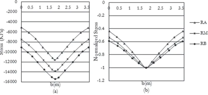
ad-opted an axial deformation modulus Ec = 32400MPa and Poisson's coefficient νc =0.2 for the concrete. For the steel it is considered Es = 200000 MPa and νs = 0.3. Once the analysis in this example is linear, it is not necessary to define the resistances of the materials. Figure 9-a shows the variations of the normal stress along the
width of the concrete slab. In these graphs, the normal stress was
obtained in the middle of the span of the beam and in the fiber above the concrete slab. In Figure 9-b, the stresses were normal
-ized regarding the peak stress in the center line of the steel profile. From Equation (1) for the effective width it is observed that the
smaller the variation of the normal stress along the width of the
slab the greater the effective width. Table 1 shows the effective width calculation. Therefore, through the graph of Figure 9-b and Table 1 it can be concluded that the effective width decreases with increasing stiffness in the connection.
Table 1 presents the effective width value according to Equation (1).
Figure 9
Variation of the normal stress along the width of the concrete slab
Table 1
Effective width
Stiffness RA RM RB
-29223.2 -37947.2 -44067.5
-11559.7 -13838.2 -15460.4
However, the effective width aims to simplify the structural analysis
of plates connected to beams maintaining the structural safety, that
is, maximum stress and displacement in the simplified structural ele
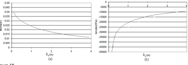
-ment, greater or equal to those found when simplification is not made. Figure 10 shows the curves that define the maximum deflection
and maximum stress in the concrete slab as a function of the slab width bv, the problem being simulated only by beam and interface elements. These curves were determined for the composite beam
of Figure 8 with RM.
With the curves of Figure 10 and the values of the maximum stress
and displacement that are obtained from the analysis of plate plus
beam, it is possible to determine the effective width of the compos -ite beam that meets the cr-iteria of maximum stress and maximum displacement. Table 2 shows the concrete beam width values of the composite beam that meet these criteria.
From Table 2 it is verified that the definition of the effective width value depends on which criterion one wishes to satisfy. For the specific example analyzed, the maximum stress criterion is less
rigorous than the maximum displacement criterion, that is, with
an effective width of the concrete slab of 2.35m the maximum displacement evaluated in the simplified analysis is equal to the
displacement in the analysis plate plus beam. However, the force
Figure 10
Composite beam stress and displacement for different values of b
vTable 2
Effective width by comparing plate analysis plus beam and beam analysis
Criteria Plate analysis plus beam bv (m)
Maximum stress (kPa) 3.21
Maximum displacement (m) 0.016 2.35
Both – 2.35
Figure 11
resulting from the normal stress distribution in the concrete slab in
the most compressed fiber evaluated in the simplified analysis is
larger than expected in the analysis of the plate plus beam,
there-fore, in favor of safety. In Table 2 it is also shown that Equation (1) for the effective width provides conservative values for the ana
-lyzed problem in relation to the criterion of maximum stress.
4.2 Composite steel-concrete
beam – nonlinear analysis
A composite beam simply supported by 3.8 m span with cross
sec-tion given by Figure 11 was collapsed through two concentrated loads equally spaced 0.5 m from the middle of the span. All experimental pro
-cedures can be seen in Amadio et al. [26]. The connection between the concrete slab and the HEB 180 Italian steel profile was made through 56 stud bolt connectors arranged in pairs and equally spaced from 10 cm from the ends of the composite beam. This configuration of the con -nection confers to the composite beam a full interaction analysis.
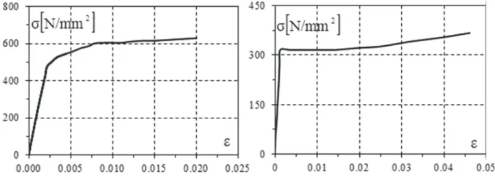
The mechanical properties of the materials were obtained through laboratory tests performed by Amadio et al. [26]. Figure 12 shows the stress-strain curves of the reinforcing bars and the steel
pro-file. In Figure 13 the result of the shear force versus slip test is
shown for a connector according to the procedure described in
Eurocode 4 [21]. In the same figure is shown a bi-linear approxima -tion for the experimental curve used in the numerical analysis of this work. The tensile and compressive strength and the axial
de-formation modulus of the concrete are, respectively, fc = 34.5 MPa,
ft = 3.32 MPa and Ec = 36744 MPa.
Figure 14 compares the numerical result obtained in this work with
the experimental result obtained by Amadio et al. [26]. In the nu -merical analysis the plate element was used to simulate the
behav-ior of the concrete slab, the beam element for the steel profile and
the interface element for the deformable connection. Due to the
symmetry of the problem, only half of the beam was discretized in finite elements, using a mesh of 6 plate elements and 3 beam and interface elements. As can be observed in Figure 14 the elements
Figure 12
Steel stress-strain curve for reinforcing bars (a) and profile (b)
Figure 13
Shear force
versus
slip for a connector
Figure 14
implemented in this work provide a good result for the composite
beam problem analyzed.
The variation of the normal stress along the width of the concrete
slab was evaluated for the composite beam analyzed at different load levels, as shown in Figure 15. As already described by other authors [3,4,26], the effective width approaches the width of the
concrete slab when the composite beam approaches the collapse.
This can be seen in the figure with the decrease of the shear lag effect as the P/Pmax ratio increases.
The number of connectors used in the connection of the concrete
slab to the steel profile of the composite beam analyzed gives to it
practically a total interaction in the mixed section. In order to
evalu-ate the degree of stiffness of the connection in the evaluation of the effective width, the same beam was numerically analyzed, assum
-ing a configuration of the connection that gives it a partial intention.
For this, the stiffness of the connection was halved, that is, instead of 56 connectors distributed in pairs, it was considered 28 connec -tors distributed in only one line. The result of the shear lag variation
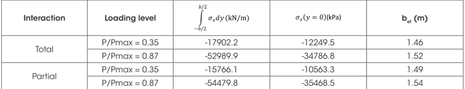
for this new connection configuration is shown in Figure 16. Figure 17-a compares, for the loading level P/Pmax = 0.35, the re
-sults obtained considering total interaction (56 connectors) and par
-tial interaction (26 connectors). The same happens in Figure 17-b for the loading level P/Pmax = 0.87. It is observed in these figures that the reduction of stiffness decreases the shear lag effect in the concrete slab, that is, the effective width is greater. Table 3 shows these effective widths obtained using Equation (1) defined above. Probably due to a large span/width ratio of the concrete slab, a small
variation of the normal stress along the width of the concrete slab
is observed, resulting in an effective width close to the width of the
concrete slab, as can be seen in Table 3. It is also observed in Table
3 that the effective width increases as the increase of the P/Pmax ratio and with the decrease in the stiffness of the connection.
Figure 15
Variation of the normal stress along the
width of the concrete slab (total interaction)
Figure 16
Variation of the normal stress along the
width of the concrete slab (partial interaction)
Figure 17
5. Conclusions
In this work the numerical analysis is used to verify the influence of the partial interaction in determining the effective width of steel-concrete composite beams. For this, the problem of composite
beam formed by a concrete slab associated with a steel beam through a deformable connection is simulated using plate, beam
and interface elements. In the first example a linear analysis of a composite beam is made considering different values for longi
-tudinal stiffness. In the second example a composite beam was brought to collapse, also considering different values for longitu
-dinal stiffness. In both cases it was possible to evaluate the rel -evance of the degree of interaction of the composite beam in
de-termining the effective width. The results show that the effective width has an inverse relation with the stiffness of the connection. In other words, the stiffer the connection the smaller the effective
width, so that the approximate analysis of the concrete slab by a bar element gives results compatible with the analysis using plate
element. This is due to the shear lag effect that is most significant for higher stiffness values. Finally, another important observation is that the effective width approaches the width of the concrete
slab when the composite beam approaches the collapse. This is evident, once the ultimate load leads to a uniform distribution of tension along the width of the concrete slab, thereby reducing the
shear lag effect and consequently increasing the effective width.
6. Acknowledgment
The authors would like to thank the Federal University of Ouro Pre
-to/PROPEC, the CNPq, and FAPEMIG, for the financial support.
7. References
[1] AMADIO C., FRAGIACOMO M. Effective width evaluation
for steel–concrete composite beams. Journal of
Construc-tional Steel Research, v.58, n.3, 2002; p. 373-388.
[2] CHIEWANICHAKORN M, AREF A.J., CHEN S.S., AHN I.S. Effective flange width definition for steel–concrete composite bridge girder. Journal of Structural Engineering, v.130, n12, 2004; p.2016-2031.
[3] CASTRO J.M., ELGHAZOULI A.Y., IZZUDDIN B.A. Assess
-ment of effective slab widths in composite beams. Journal of Constructional Steel Research, v.63, 2007; p.1317-1327.
[4] NIE J-G., TIANA C-Y, CAIB C.S. Effective width of steel–con
-crete composite beam at ultimate strength state. Engineer
-ing Structures, v.30, 2008; p.1396-1407.
[5] AHN I1-S., CHIEWANICHAKORN M., CHEN S. S., AREF A. J. Effective flange width provisions for composite steel bridges. Engineering Structures, v.26, 2004; p.1843-1851 [6] ADEKOLA A. O. Effective width of composite beams of
steel and concrete. The Structural Engineer. v.46, n.9, 1968;
p.285-294.
[7] ALLEN D. N. G., SEVERN R. T. Composite action between beams and slabs under transverse load. The Structural En
-gineer v.39, Part I, 1961; p.149-54.
[8] ANSOURIAN P. An application of the method of finite elements to the analysis of composite floor systems. Proceedings of the Institution of Civil Engineers. v.59, 1975; p.699-726.
[9] ANSOURIAN P., AUST M. I. E. The effective width of contin
-uous composite beams. Civil Engineering Transitions v.25, n.1, 1983; p.63-72.
[10] HEINS C.P., FAN H.M. Effective composite beam width at ul
-timate load. Journal of Structural Division, ASCE v.102, n.11, 1976; p.2163-2179.
[11] ELKELISH S., ROBINSON H. Effective widths of composite beams with ribbed metal deck. Canadian Journal of Civil En
-gineering v.13, n.5, 1986; p.75-82.
[12] AMADIO C., FEDRIGO C., FRAGIACOMO M., MACORINI L. Experimental evaluation of effective width in steel–con -crete composite beams. Journal of Constructional Steel
Re-search 60, 2004; p.199-220.
[13] ABAQUS (2008). Standard user’s manual. 6.8-1. ed. USA:
Hibbitt, 2008.
[14] FAHMY E. H., ROBINSON H. Analyses and tests to deter
-mine the effective widths of composite beams in unbraced multistory frames. Journal of Civil Engineering v.13, n.1 1986; p.66-75.
[15] SILVA A. R. Numerical Analysis of Structural Elements with Partial Interaction, Ouro Preto, 2010, Doctoral Thesis, Post-graduation Program in Civil Engineering, Federal University of Ouro Preto, 180 p.
[16] BATHE, K. J. Finite element procedures, Prentice-Hall, En
-glewood Cliffs, 1996, 1037 p.
[17] HUANG Z. BURGESS I.W., PLANK R.J. Modelling Mem -brane Action of Concrete Slabs in Composite Buildings in
Fire. Part I: Theoretical Development. Journal of Structural Engineering, ASCE. v.129, n.8, 2003a; p.1093-1102.
Table 3
Effective width
Interaction Loading level bef (m)
Total P/Pmax = 0.35 -17902.2 -12249.5 1.46
P/Pmax = 0.87 -52989.9 -34786.8 1.52
Partial P/Pmax = 0.35 -15766.1 -10563.3 1.49
brane Action of Concrete Slabs in Composite Buildings in
Fire. Part II: Validations. Journal of Structural Engineering, ASCE. v.129 n.8, 2003b; p.1103-1112.
[20] AMERICAN SOCIETY OF CIVIL ENGINEERS (ASCE). Finite element analysis of reinforced concrete. New York, 1982. [21] COMITE EUROPEEN DE NORMALISATION. Design of com
-posite steel and concrete structures part I: general rules and
rules for buildings. – EUROCODE 4, Brussels, Belgium, 2004.
[22] SOUSA JR. J. B. M., SILVA, A. R. Nonlinear analysis of partially
connected composite beams using interface elements. Finite Elements in Analysis and Design. v.43, 2007; p.954-964.
[23] SILVA A. R., SOUSA JR J. B. M. A family of interface ele-ments for the analysis of composite beams with interlayer
slip. Finite Elements in Analysis and Design. v.45, 2009;
p.305-314.
[24] SOUSA JR J. B. M., CLÁUDIO E. M. O., SILVA A. R. Non -linear analysis of partially connected composite beams us-ing interface elements. Journal of Constructional Steel
Re-search. v.6, 2010; p.772-779.
[25] OLLGAARD, J. G., SLUTTER, R. G., FISHER, J. W. Shear
strength of stud connectors in lightweight and normal-weight
concrete. AISC Engineering Journal. 1971; p.55-64. [26] AMADIO C., FEDRIGO C. Experimental evaluation of Ef
-fective width in steel–concrete composite beams. Journal of