Correlation between seismicity and barometric tidal exalting

(1)

www.nat-hazards-earth-syst-sci.net/8/1129/2008/ © Author(s) 2008. This work is distributed under the Creative Commons Attribution 3.0 License.

and Earth

System Sciences

Correlation between seismicity and barometric tidal exalting

D. N. Arabelos1, G. Asteriadis1, A. Bloutsos2, M. E. Contadakis1, and S. D. Spatalas1

1_{Department of Geodesy and Surveying, Aristotle University of Thessaloniki, 54124, Thessaloniki, Greece} 2_{Department of Meteorology and Climatology, Aristotle University of Thessaloniki, 54124, Thessaloniki, Greece}

Received: 6 June 2008 – Revised: 4 September 2008 – Accepted: 4 September 2008 – Published: 21 October 2008

Abstract. Changes of barometric pressure in the area of Thessaloniki in Northern Greece were studied by analyzing a sample of 31 years of hourly measurements. The results of this analysis on the periodicities of tidal components are ex-pressed in terms of amplitude and phases variability. An ear-lier investigation revealed a detectable correlation between the exalting of the amplitude parameters of the tidal waves with strong seismic events. A problem of this work was that we had compared the tidal parameters resulting from the analysis of data covering the period of one year with instan-taneous seismic events, although the earthquake is the final result of a tectonic process of the upper lithosphere. Con-sequently, in order to increase the resolution of our method we had analyzed our data in groups of 3-months extent and the resulted amplitudes were compared with seismicity in-dex for corresponding time periods. A stronger correlation was found in the last case. However, the estimation of tidal parameters in this case was restricted to short period (from one day down to eight hours) constituents. Therefore, a new analysis was performed, retaining the one-year length of each data block but shifting the one year window by steps of three months from the beginning to the end of the 31 years period. This way, we are able to estimate again tidal parameters rang-ing from periods of one year (Sa) down to eight hours (M3). The resulting correlation between these tidal parameters with a cumulative seismicity index for corresponding time inter-vals was remarkably increased.

1 Introduction

It is broadly accepted and well documented that a number of physical phenomena and respectively a number of phys-ical parameters present unusual behavior during the

earth-Correspondence to:D. N. Arabelos (arab@eng.auth.gr)

quake preparation period as well as during the earthquake itself (e.g. Rikitake, 1981; Hayakawa, 1999; Hayakawa and Molchanov, 2002). The understanding of the intriguing way in which these phenomena are connected with the tectonic activity through the lithosphere-atmosphere-ionosphere cou-pling, is a challenging task by itself. In addition, due to the vast cost in lives and in social economy of a potential strong earthquake it has become imperative to investigate these phenomena in order to render any meaningful infor-mation about their connection with disastrous events and use the acquired knowledge for the effective mitigation of seis-mic hazard. Apart of the pure seismological research, a vast amount of research is currently carried out on a number of observables connected with these phenomena. A lot of atmo-spheric physical parameters i.e. density, ionoatmo-spheric ion con-tent, electromagnetic field, EM transmissivity etc., varies in a mutual interaction with lithospheric and ionospheric vari-ations (e.g. Hayakawa et al., 1996; Silina et al., 2001; Ma-reev et al., 2002; Biagi et al., 2003; Molchanov et al., 2003, 2004; Plotkin, 2003). It could be used to detect extreme litho-spheric variations, like the ones related to earthquakes. That requires a careful and very often sophisticated analysis to re-move the inherent noise.

(2)

Atmospheric tides in the area of Thessaloniki were earlier studied by analyzing an 11 years sample of hourly baromet-ric measurements (Arabelos et al., 1997). In an earlier pa-per by Biagi et al. (2003) the presence of tidal harmonics in the spectral content of three LF radio signals was reported indicating that atmospheric process with tidal periodicities are one of the factors affecting the propagation of LF radio waves. In addition they reported anomalous increase in the intensity of the radio signals which was propagated over the epicenter of a seismic sequence in Slovenia during the last month before the beginning of the sequence. They suggested that preseismic exalting of the atmospheric tides, produced by a gravity decrease due to fluid diffusion in a broad area around the epicenter, was responsible for the radio signal ex-alting. In a recent paper, Molchanov et al. (2004) present a general concept of mechanisms of preseismic phenomena in the atmosphere and ionosphere. Among them, they con-cluded that atmospheric perturbation of temperature and den-sity could follow preseismic hot water/gas release near the ground surface. On the other hand, atmospheric tides depend on the atmospheric temperature and density (Chapman and Lindzen, 1970). Thus, if this concept is true, an alteration of the atmospheric tides, or at least of some constituent of them, is to be expected in the area of increased seismic ac-tivity around the time of its occurrence. These facts render the hope that observables related to atmospheric tides may probably be used as earthquake precursory phenomena (Gor-baticov et al., 1999).

Thessaloniki, being 30 km southeastern of the very active seismic area of Volvi and Langada lakes, is located under the threat of a potentially large earthquake. Therefore, a pro-gram for the investigation of a possible correlation of the at-mospheric tides parameters with seismic activity in the area of Thessaloniki was initiated. The first results of this investi-gation (Arabelos et al., 2003, 2004) indicate a correlation of the annual variation of some wave groups with the seismic activity around Thessaloniki. This was shown by plotting the variations of the tidal amplitude of these wave groups to-gether with individual earthquakes occurred around the test area.

In the present paper we investigate the variations of the tidal parameters of the barometric pressure in relation with the seismic activity in an extended area around Thessaloniki. A cross-correlation analysis of the tidal amplitude variations of certain wave groups with the seismicity of the area re-sulted in a quantitative consideration of this relation. The choice of the tidal waves considered is this work was based on their signal to noise ratio, regardless of their origin. Note that the aim of this work was to investigate possible correla-tion between seismicity and barometric tidal exalting, with-out attempting explanation of this coupling. Furthermore, it should be mentioned that with its present low resolution our method could not be applicable to forecast occurrence of earthquakes.

2 Observational material and model of normal

potential

In the present analysis the data sets used were the following: Model of tidal potential

From the models of Normal Tidal Potential we chose that of Tamura (1987) which includes 1200 waves.

Barometric pressure and temperature data for the area of Thessaloniki

The atmospheric pressure has been recorded with the help of a membrane box barograph and corrected with the help of a mercury pipe barometer installed in the same place with the barograph. The accuracy of each measurement of pressure is±1 hPa. The data set includes 267 984 hourly values of the barometric pressure covering the period from 1 January 1975 to 31 December 2005 (11 166 days totally). These val-ues have been derived from analogue registrations in the Me-teorological Station of the Department of Meteorology and Climatology of the Aristotle University of Thessaloniki. The data set was used for the determination of the atmospheric modulations.

The atmospheric temperature was recorded with the help of a bimetallic thermograph and a mercury thermometer. The precision of each measurement of temperature is±0.1◦_C.

The hourly values of the temperature for the same period as in the section on barometric pressure data have been used to estimate the correlation between atmospheric temperature close to the earth’s surface and barometric pressure.

Earthquake catalogue

The catalogue of the Geodynamic Institute/National Obser-vatory of Athens was used, including 43 128 earthquakes from 1964 up to now, occurred in the area bounded by 33.47◦≤ϕ≤42.20◦,16.26◦≤λ≤30.36◦. The local magnitude of these events varies fromML=1.4 toML=7. In the next this would be referred as NOA catalogue.

3 Analysis of the barometric measurements and

com-putation of a seismicity index

(3)

information resulting from our method might be useful if the correlation is concerned with shorter period.

In the afore-mentioned earlier papers the estimated annual values of the amplitude of 22 wave groups, resulting from the analysis of hourly barometric measurements covering the period from 1975 to 2005 (31 years), were plotted together with the earthquakes withM≥4 occurred at the same period, up to a distance of 200 km from Thessaloniki. The figures produced in this way showed a significant correlation in the case of some groups such as Sa and Ssa, while in some other cases the situation was confusing.

In order to be able to evaluate this correlation, it was nec-essary to compare the changes of the amplitude of the tidal waves with a “seismicity index” such as the seismic energy E, according to

log10ES=a+bMS, (1)

wherea, b are constants andMS is the surface magnitude of the earthquake. Since the computed amplitude values of the tidal waves are practically annual mean values the com-parison should carried out with the cumulative energyKfor corresponding time intervals

Ki =

t2

X

t1

(ES)ψ≤R, (2)

whereψis the distance of the earthquake epicenter from the barometric station,R is the maximum distance up to which earthquakes were taken into account andt1, t2define the

cor-responding annual time intervali. The estimation ofRwas based on some numerical experiments as it will be discussed later on. For the constants a and b of Eq. (1) the values 4.8 and 1.5, respectively, were suggested by Gutenberg and Richter (1956). The value 4.8 for the coefficientawas con-sidered as overestimated by Choy and Boatwright (1995). They suggest the valuea=4.4 resulting from a global set of 397 earthquakes. However, the choice ofais not critical for our analysis, since Eq. (1) is linear. On the other hand, for the coefficientb which is critical for our analysis there is a general agreement between the authors.

Since for the estimation of Eq. (1) the surface magnitude MS of the earthquakes is needed, it was necessary to trans-form the local magnitudeMLincluded in the NOA catalogue to corresponding surface one. For this purpose the equation

MS =c+dML, (3)

was used, wherec, dconstants. For the evaluation of Eq. (3) the values ofc=−3.35±0.263 andd=1.687±0.053 were de-fined by Tzanis and Vallianatos (2003) after a sophisticated comparison of 1184 common events between 1 January 1978 and 30 April 2000, contained in the NOA-ML and the In-ternational Seismological Centre (ISC)-MS catalogues. Fol-lowing the authors the two magnitude scales are apparently linearly correlated forMS>3 and ML>3.4−3.5. In a new attempt we tried to define the constantscandd, using the

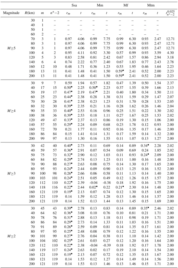
available common events of NOA-MLand ISCMS, between 1 January 1978 and 31 December 2006. A number of 1416 common events were identified, allowing differences in time up to 8 s and up to 0.2 degrees in the latitude/longitude coor-dinates (not simultaneously at the same record). The linear regression model (Eq. 3) was used for the comparison of the magnitudes, resulting in the valuesc=−1.5499, d=1.2565 with a relatively low coefficient of determinationr2=0.608. In Table 1 the statistics of the differences M_SISC−M_SNOA is shown, whereM_SNOA=c+dM_LNOA.

The statistics in both cases, either using the constants by Tzanis and Vallianatos (2003) or the computed in the present work are very close. The small differences shown in Ta-ble 1 are due to the fact that the constants by Tzanis and Vallianatos (2003) have been used practically to extrapolate the additional data used for the determination of the coeffi-cients of the present work. However these results could not be considered satisfactory for this study. Therefore, we de-cided to avoid transformation ofMLtoMSand to substitute the radiated energyESby a seismicity index (e.g. Tzanis and Vallianatos, 2003)

log10=a+bM, (4)

wherea, b are constants and M is the local magnitude of the earthquake. For the evaluation of Eq. (4) the values suggested by Gutenberg and Richter (1956), i.e.a=4.8 and b=1.5 were used for the reason discussed previously. The comparison with the computed annual mean values of the tidal waves was carried out with the cumulative values of the indexCfor corresponding time intervals according to Ci =

t2

X

t1

log10()ψ≤R. (5)

To estimate tidal parameters for periods ranging from half a year (Ssa) down to eight hours (M3) and simultaneously to keep a reasonable resolution, we performed the analysis of the barometric data in blocks, retaining the one year length of each block and using a shift of this window by a three months step from the beginning to the end of the time se-ries. Note that performing the analysis in this way, smoothed amplitude changes were resulted instead of the actual ones. This was a necessary compromise though, for the method of analysis followed. Consequently, the summation fromt1

tot2in Eq. (5) was extended for corresponding intervals of

(4)

Table 1. Statistics of the differences betweenM_SISCandM_SNOA, based on the estimated constantscanddof Eq. (3).

Mean Standard Minimum Maximum

Constants No value deviation difference difference

c=−3.350,d=1.687 1416 −0.072 0.512 −1.591 3.071

c=−1.485,d=1.242 1416 0.000 0.471 −1.353 2.950

0 1 2 3 4 5 6 7 8 9 10 11 12 13 14 15

Cumulative seismicity index C

1977 1980 1983 1986 1989 1992 1995 1998 2001 2004

Time (yr) 0

1 2 3 4 5 6 7 8 9 10 11 12 13 14 15

Cumulative seismicity index C

1977 1980 1983 1986 1989 1992 1995 1998 2001 2004

Time (yr)

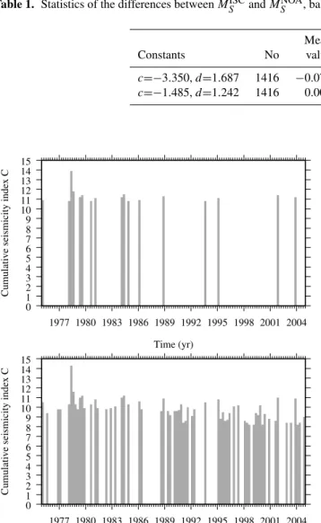
Fig. 1. Cumulative values ofC, computed for earthquakes up to a distance of 40 km from Thessaloniki taking into account earth-quakes withM≥2 (lower part) orM≥4 (upper part).

belongs to this sequence. The smaller values ofCare due to rather isolated events (1 to 2 shocks).

Using the time series of hourly values of the barometric pressure with annual extent it is possible to estimate tidal pa-rameters for periods of half a year (Ssa) down to eight hours. In order to exclude the case that the barometric tide distur-bances are due to changes of the atmospheric temperature close to the earth’s surface, the correlation between baromet-ric tides and atmosphebaromet-ric temperature was estimated using a similar data set of hourly atmospheric temperature values. A linear regression model was used for this purpose. Then, the correlated part was subtracted from the original observation. In Fig. 2, the correlation of the barometric changes with the

-0.70 -0.65 -0.60 -0.55 -0.50 -0.45 -0.40 -0.35 -0.30 -0.25 -0.20 -0.15 -0.10 -0.05 0.00 0.05 0.10

hPa/

oC

1977 1980 1983 1986 1989 1992 1995 1998 2001 2004 Time (yr)

-0.70 -0.65 -0.60 -0.55 -0.50 -0.45 -0.40 -0.35 -0.30 -0.25 -0.20 -0.15 -0.10 -0.05 0.00 0.05 0.10

hPa/

oC

1977 1980 1983 1986 1989 1992 1995 1998 2001 2004 Time (yr)

Fig. 2. Correlation between the barometric changes and atmo-spheric temperature computed for each annual group of observa-tions separately (blue line). The red line corresponds to the correla-tion computed for the entire period of the 31 years.

atmospheric temperature is shown computed for each of the 121 groups of observations separately. The accuracy of this estimation ranges from 0.001 to 0.01 hPa/◦C. Tidal param-eters were estimated for 18 tidal waves for each of the 121 groups of observations but only the parameters of 7 waves were used in the correlation analysis which will be described in the next section, since the signal to noise ratio was very weak (below 1.0 in average) for the rest. In Table 2, the mean, minimum and maximum of the 121 values of signal to noise ratio are shown for only these 7 tidal waves, which are the basis of our correlation analysis. These values are based on least square analysis. In Fig. 3 the changes of the tidal amplitude of Ssa and Mm are shown.

4 Cross-correlation analysis

The cross-correlation between the amplitude of the tidal waves designated byAi and the seismicity index Ci, was computed using the well known formula (e.g. Davis, 1973)

rm= n

∗P_A

iCi−PAiPCi

{[n∗P

A2_i −(P

Ai)2_][_n∗P

C_i2−(P

Ci)2_]}1/2,

(5)

Table 2. Mean, minimum and maximum values of signal to noise ratio for each tidal wave estimated for the 121 groups of observa-tions based on least squares analysis.

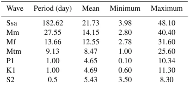
Wave Period (day) Mean Minimum Maximum

Ssa 182.62 21.73 3.98 48.10

Mm 27.55 14.15 2.80 40.40

Mf 13.66 12.55 2.78 31.60

Mtm 9.13 8.47 1.00 25.60

P1 1.00 4.65 0.10 10.34

K1 1.00 4.69 0.60 11.30

S2 0.5 5.43 3.50 8.30

wherermthe cross-correlation coefficient for match position mandn∗ the number of overlapped positions between the two chains.

The significance of the cross-correlation coefficient can be assessed by the approximate test

t=rm

_n∗₋₂

1−r2

m 1/2

, (7)

which has(n∗−2)degrees of freedom. This test was derived from a test for the significance of the correlation between two samples drawn from normal populations. The null hypothe-sis is that the correlation is zero. The algorithm used slides the first chain past the second one, computing successive val-ues ofrmand corresponding values oft for overlapped seg-ments ofn∗≥3 because there are no degrees of freedom for n∗<3. In this work we present values ofrmandtonly for the complete overlapping of the two chains under consideration. The cross-correlation was computed taking into account earthquakes of different magnitude and in different distances from the barometric pressure station. More specifically, the seismicity index was computed taking into account (i) earth-quakes with M≥2, M≥3, M≥4 and M≥5 and (ii) for all cases of (i), including for the computation ofCearthquakes up to distances ranging from 30 up to 250 km from the baro-metric pressure station. The correlation was computed ig-noring quiet periods (withC=0). If these periods were in-cluded in the analysis the correlation coefficients will result in considerably reduced values. A plausible explanation of this could be that there are many other causes influencing the changes of the barometric pressure.

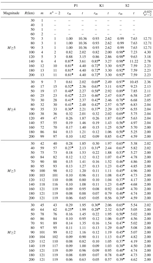
In Table 3 the statistical data of the cross-correlation anal-ysis for seismicity index including earthquakes up to a ra-diusR=200 km from the barometric station are shown for the long period wavesSsa, Mm, Mf and Mtm. The cor-responding statistical data for the short period waves P1, K1 and S2 are shown in Table 4. Correlation coefficients marked with a•are passing the statistical test of significance. In both tables the critical valuest_n0∗.025₋₂ are shown in the last column.

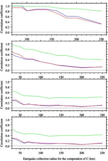
In Figs. 4 and 5 the changes of the correlation coefficient

0 1 2 3 4 5

Tidal amplitude (hPa)

1977 1980 1983 1986 1989 1992 1995 1998 2001 2004

Time (yr) 0

1 2 3 4 5

Tidal amplitude (hPa)

1977 1980 1983 1986 1989 1992 1995 1998 2001 2004

Time (yr)

Fig. 3.Changes of the amplitude of Ssa (blue) and of Mm (red) of the 121 annual groups of hourly barometric observations.

with the distance up to R=250 km are shown for the long and short period waves, respectively. Note that forM≥5,C is computed starting from a collection radius of 70 km, since there are very few events in shorter distances from Thessa-loniki, during the entire period considered. Therefore, the distance scale forM≥5 is different than the corresponding in the other diagrams.

In Table 3 and Fig. 4 it is shown that forM≥5 consid-erable correlation coefficients are resulting for values ofC computed with a collection radius up to 150 km from the barometric pressure station. These correlation coefficients failed to pass thet-test for significance level equal to 0.05. However, the degrees of freedom are not statistically suffi-cient up to a distance of 160 km from the barometric station. By increasing the collection radius the correlation becomes weaker and practically vanishes after the distance of about 150 km. Furthermore, the correlation becomes weaker forC including earthquakes withM≥4,M≥3 andM≥2, although larger values ofCresulted in these cases. From this point of view it might be concluded that distant or weak earthquakes are not correlated with the seismicity of the test area and consequently they behave as noise, decreasing in this way the overall correlation. Note that the correlation coefficients for Ssa are passing thet-test, for seismicity index computed from earthquakes withM≥4,M≥3 andM≥2 collected up to 150 km from the barometric station.

(6)

0.0 0.2 0.4 0.6 0.8 1.0 Correlation coefficient

50 100 150 200 250

Earthquake collection radius for the computation of C (km) 0.0 0.2 0.4 0.6 0.8 1.0 Correlation coefficient

50 100 150 200 250

0.0 0.2 0.4 0.6 0.8 1.0 Correlation coefficien

50 100 150 200 250

100 150 200 250

Fig. 4. Correlation coefficients between the amplitude of long pe-riod waves Ssa (blue), Mm (red), Mf (green) and Mtm (gray) and the seismicity indexC. From the bottom to the top: Ccomputed including earthquakes withM≥2, M≥3, M≥4 andM≥5.

of the short period waves is promising for an increase of the resolution of this method, because the estimation of tidal pa-rameters of the barometric pressure for the diurnal and semi-diurnal waves is possible using time series of much shorter extend than those needed for the long period waves.

5 Conclusion

The analysis of the barometric tides in the area of Thessa-loniki showed a clear correlation between the disturbances of the amplitude of some long period wave groups with the seismicity of the test area resulting from earthquakes with M≥5 up to distance of about 150 km from the barometric station. For earthquakes withM≥4 the correlation is rapidly decreasing and practically vanishes after a distance of about 50 to 60 km from the barometric station.

Considerable values of correlation are also observed in the case of some diurnal and semi-diurnal waves, with

domi-0.0 0.2 0.4 0.6 0.8 1.0 Correlation coefficient

50 100 150 200 250

Eartquake collection radius for the computation of C (km) 0.0 0.2 0.4 0.6 0.8 1.0 Correlation coefficient

50 100 150 200 250

100 150 200 250

Fig. 5.Correlation coefficients between the amplitude of short pe-riod waves P1 (blue), K1 (red) and S2 (green) and the seismicity indexC. From the bottom to the top:Ccomputed including earth-quakes withM≥2, M≥3, M≥4 andM≥5.

nant the case of S2, where significant values of correlation resulted even for distances up to 200 km from the barometric station.

The correlation in general becomes weaker by increasing the radius of earthquakes collection for the computation of the seismicity index. On the other hand, the correlation be-comes weaker as earthquakes with small magnitude are in-cluded in the computation of the seismicity index, although the seismicity index is increasing. This behavior allows us to conclude that distant (even strong) earthquakes or weak earthquakes (even very close to the test area) are not corre-lated with the tidal changes of the barometric pressure.

(7)

Table 3. Results of the cross-correlation analysis for the long period waves Ssa, Mm, Mf and Mtm. The indexmofrdenotes the number of terms matched, which in our case coincides with the numberNofC>0 in each chain. In additionNmust be at least 3 in order to fulfill the conditionn∗≥3. The seismicity indexCwas computed including earthquakes withM≥5,M≥4,M≥3 andM≥2. Correlation coefficients marked by a•are passing thet-test for significance level equal to 0.05.

Ssa Mm Mf Mtm

Magnitude R(km) m n∗−2 rm t rm t rm t rm t t_n0∗.025₋₂

30 1 – – – – – – – – –

40 1 – – – – – – – – –

50 1 – – – – – – – – –

60 2 – – – – – – – – –

70 3 1 0.97 4.06 0.99 7.75 0.99 6.30 0.93 2.47 12.71

80 3 1 0.97 4.06 0.99 7.75 0.99 6.30 0.93 2.47 12.71

M≥5 90 3 1 0.97 4.06 0.99 7.75 0.99 6.30 0.93 2.47 12.71

100 4 2 0.95 4.11 0.92 3.30 0.57 0.99 0.93 3.59 4.30

120 5 3 0.83 2.58 0.81 2.42 0.67 1.57 0.86 2.94 3.18

140 6 4 0.74 2.22 0.77 2.40 0.67 1.83 0.77 2.43 2.78

160 12 10 0.48 1.71 0.36 1.23 0.53 1.95 0.46 1.64 2.23

180 13 11 0.41 1.48 0.41 1.50 0.59• 2.41 0.52 2.00 2.23

200 13 11 0.41 1.48 0.41 1.50 0.59• 2.41 0.52 2.00 2.23

30 9 7 0.59 1.94 0.57 1.82 0.47 1.39 0.50 1.54 2.37

40 17 15 0.50• 2.25 0.50• 2.23 0.37 1.55 0.39 1.66 2.13

50 19 17 0.47• 2.19 0.47• 2.21 0.40 1.80 0.34 1.50 2.11

60 25 23 0.44• 2.38 0.28 1.38 0.31 1.59 0.29 1.47 2.07

70 30 28 0.41• 2.38 0.23 1.23 0.31 1.70 0.28 1.53 2.05

80 32 30 0.39• 2.35 0.21 1.16 0.28 1.62 0.26 1.46 2.04

M≥4 90 35 33 0.40• 2.53 0.16 0.96 0.25 1.51 0.22 1.30 2.02

100 38 36 0.39• 2.53 0.18 1.11 0.27 1.67 0.25 1.53 2.02

120 49 47 0.33• 2.37 0.13 0.86 0.19 1.30 0.15 1.06 2.00

140 57 55 0.29• 2.24 0.09 0.68 0.23 1.78 0.12 0.93 2.00

160 72 70 0.21 1.77 0.11 0.92 0.16 1.35 0.17 1.46 2.00

180 86 84 0.15 1.41 0.14 1.31 0.17 1.59 0.14 1.32 2.00

200 99 97 0.13 1.30 0.16 1.55 0.11 1.07 0.13 1.27 2.00

30 42 40 0.40• 2.73 0.11 0.69 0.14 0.89 0.34• 2.28 2.02

40 59 57 0.36• 2.91 0.07 0.54 0.09 0.69 0.24 1.85 2.02

50 75 73 0.32• 2.90 0.12 1.03 0.11 0.93 0.24• 2.09 2.00

60 84 82 0.29• 2.74 0.13 1.23 0.11 1.00 0.16 1.48 2.00

70 90 88 0.27• 2.63 0.08 0.75 0.14 1.30 0.17 1.65 2.00

80 95 93 0.24• 2.44 0.09 0.90 0.13 1.25 0.16 1.52 2.00

M≥3 90 100 98 0.26• 2.66 0.06 0.58 0.11 1.13 0.14 1.40 2.00

100 103 101 0.24• 2.51 0.05 0.49 0.12 1.26 0.15 1.57 2.00

120 112 110 0.22• 2.39 -0.04 -0.38 0.18 1.92 0.16 1.75 2.00

140 118 116 0.22• 2.44 0.02• 0.22 0.21• 2.30 0.14 1.48 2.00

160 121 119 0.19• 2.13 0.07 0.74 0.12 1.30 0.15 1.65 2.00

180 121 119 0.14 1.59 0.12 1.28 0.13 1.46 0.14 1.57 2.00

200 121 119 0.14 1.52 0.13 1.44 0.13 1.45 0.15 1.69 2.00

30 45 43 0.39• 2.78 0.13 0.83 0.14 0.89 0.35• 2.46 2.02

40 64 62 0.36• 3.08 0.10 0.76 0.10 0.81 0.21 1.71 2.00

50 78 76 0.31• 2.88 0.13 1.18 0.11 0.98 0.19 1.71 2.00

60 86 84 0.29• 2.73 0.14 1.33 0.11 1.03 0.16 1.51 2.00

70 91 89 0.26• 2.59 0.09 0.81 0.14 1.35 0.17 1.61 2.00

80 97 95 0.25• 2.48 0.08 0.79 0.12 1.22 0.16 1.55 2.00

M≥2 90 101 99 0.27• 2.76 0.04 0.38 0.11 1.10 0.14 1.42 2.00

100 104 102 0.25• 2.61 0.03 0.27 0.12 1.20 0.16 1.64 2.00

120 112 110 0.22• 2.38 -0.04 -0.39 0.18 1.92 0.17 1.78 2.00

140 119 117 0.24• 2.63 0.02 0.17 0.19 2.10 0.14 1.54 2.00

160 121 119 0.19• 2.13 0.07 0.72 0.12 1.35 0.15 1.67 2.00

180 121 119 0.14 1.53 0.12 1.27 0.14 1.49 0.14 1.56 2.00

(8)

Table 4. Results of the cross-correlation analysis for the short period waves P1, K1 and S2. The indexmofrdenotes the number of terms matched, which in our case coincides with the numberN ofC>0 in each chain. In additionN must be at least 3 in order to fulfill the conditionn∗≥3. The seismicity indexCwas computed including earthquakes withM≥5,M≥4,M≥3 andM≥2. Correlation coefficients marked by a•are passing thet-test for significance level equal to 0.05.

P1 K1 S2

Magnitude R(km) m n∗−2 rm t rm t rm t t_n0∗.025₋₂

30 1 – – – – – – –

40 1 – – – – – – –

50 1 – – – – – – –

60 2 – – – – – – –

70 3 1 1.00 10.36 0.93 2.62 0.99 7.63 12.71

80 3 1 1.00 10.36 0.93 2.62 0.99 7.63 12.71

M≥5 90 3 1 1.00 10.36 0.93 2.62 0.99 7.63 12.71

100 4 2 0.82 2.02 0.82 2.00 0.98• 7.23 4.30

120 5 3 0.88 3.15 0.86 2.86 0.98• 9.63 3.18

140 6 4 0.87• 3.61 0.85• 3.27 0.98• 11.22 2.78

160 12 10 0.81• 4.40 0.72• 3.30 0.92• 7.59 2.23

180 13 11 0.81• 4.40 0.72• 3.30 0.92• 7.59 2.23

200 13 11 0.81• 4.40 0.72• 3.30 0.92• 7.59 2.23

30 9 7 0.61 2.02 0.69• 2.49 0.97• 10.45 2.36

40 17 15 0.52• 2.36 0.63• 3.11 0.92• 9.23 2.13

50 19 17 0.48• 2.27 0.58• 2.92 0.89• 7.85 2.11

60 25 23 0.42• 2.23 0.46• 2.47 0.81• 6.58 2.07

70 30 28 0.41• 2.37 0.42• 2.46 0.78• 6.68 2.05

80 32 30 0.41• 2.48 0.42• 2.57 0.78• 6.83 2.04

M≥4 90 35 33 0.36• 2.21 0.37• 2.29 0.75• 6.55 2.04

100 38 36 0.32 2.01 0.32 2.02 0.69• 5.75 2.04

120 49 47 0.26 1.87 0.26 1.87 0.63• 5.63 2.04

140 57 55 0.19 1.46 0.19 1.43 0.56• 4.97 2.04

160 72 70 0.17 1.40 0.15 1.25 0.56• 5.70 2.00

180 86 84 0.13 1.21 0.12 1.06 0.50• 5.25 2.00

200 99 97 0.10 1.02 0.09 0.85 0.42• 4.59 2.00

30 42 40 0.28 1.85 0.30 1.97 0.65• 5.38 2.02

40 59 57 0.27• 2.13 0.31• 2.44 0.61• 5.82 2.02

50 75 73 0.18 1.53 0.22 1.88 0.53• 5.27 2.00

60 84 82 0.12 1.12 0.12 1.07 0.47• 4.78 2.00

70 90 88 0.15 1.41 0.16 1.52 0.46• 4.86 2.00

80 95 93 0.13 1.27 0.13 1.23 0.45• 4.85 2.00

M≥3 90 100 98 0.12 1.20 0.11 1.11 0.45• 4.96 2.00

100 103 101 0.10 0.96 0.11 1.08 0.43• 4.73 2.00

120 112 110 0.08 0.80 0.10 1.04 0.37• 4.17 2.00

140 118 116 0.10 1.08 0.11 1.23 0.40• 4.68 2.00

160 121 119 0.09 0.95 0.08 0.92 0.40• 4.70 2.00

180 121 119 0.08 0.88 0.07 0.79 0.40• 4.74 2.00

200 121 119 0.06 0.65 0.05 0.56 0.39• 4.59 2.00

30 45 43 0.29 1.95 0.30• 2.06 0.65• 5.54 2.02

40 64 62 0.25• 1.99 0.28• 2.32 0.54• 5.05 2.00

50 78 76 0.16 1.45 0.22 1.95 0.50• 5.02 2.00

60 86 84 0.10 0.95 0.12 1.06 0.45• 4.56 2.00

70 91 89 0.14 1.35 0.16 1.54 0.47• 5.02 2.00

80 97 95 0.11 1.11 0.13 1.29 0.46• 5.08 2.00

M≥2 90 101 99 0.12 1.16 0.12 1.19 0.45• 5.07 2.00

100 104 102 0.09 0.90 0.11 1.13 0.43• 4.82 2.00

120 112 110 0.08 0.82 0.10 1.05 0.37• 4.19 2.00

140 119 117 0.09 1.00 0.09 1.03 0.38• 4.50 2.00

160 121 119 0.09 0.96 0.09 0.95 0.40• 4.74 2.00

180 121 119 0.08 0.89 0.07 0.78 0.40• 4.73 2.00

(9)

Our results may be considered to be consistent, or at least not contradicting with the general concept of the mechanisms of preseismic phenomena in the atmosphere and ionosphere discussed in Sect. 1. According to this concept precursory phenomena such as atmospheric perturbations of tempera-ture, density etc., result from an upward migration of fluid substrate matter in the strength-weakened areas of the crust.

Acknowledgements. We are very thankful for the important

comments by the reviewers, helping us to improve the paper.

Edited by: M. Contadakis

Reviewed by: P. F. Biagi and another anonymous referee

References

Arabelos, D., Asteriadis, G., Contadakis, M. E., Spatalas, S. D., and Sachsamanoglou, H.: Atmospheric tides in the area of Thes-saloniki, J. Geodyn., 23, 65–75, 1997.

Arabelos, D., Asteriadis, G., Bloutsos, A., Contadakis, M. E., Kalt-sikis, Ch., and Spatalas, S. D.: Atmospheric tides in the area of Thessaloniki-North Greece. A twenty-seven years data analysis, From Stars to Earth and Culture, In honour of the memory of Professor Alexandros Tsioumis, edited by: Dermanis, A., Pub-lishing Ziti, Thessaloniki, 201–207, 2003.

Arabelos, D. N., Asteriadis, G., Bloutsos, A., Contadakis, M. E., and Spatalas, S. D.: Atmospheric tide disturbances as Earthquake precursory phenomena, Nat. Hazards Earth Syst. Sci., 4, 1–7, 2004, http://www.nat-hazards-earth-syst-sci.net/4/1/2004/. Bartzokas, A.: Dynamical factors influencing the daily barometric

fluctuation in the vicinity of the ground, in the area of Greece, Ph.D. Thesis, University of Ioannena, Greece, 208 pp., 1989. Bartzokas, A., Repapis, C. C., and Metaxas, D. A.: Temporal

varia-tions of atmospheric tides over Athens, Meteorol. Atmos. Phys., 55, 113–123, 1995.

Biagi, P. F., Piccolo, R., Capozzi, V., Ermini, A., Martellucci, S., and Bellecci, C.: Exalting in atmospheric tides as earthquake precursor, Nat. Hazards Earth Syst. Sci., 3, 197–201, 2003, http://www.nat-hazards-earth-syst-sci.net/3/197/2003/.

Chapman, S. and Lindzen, R. S.: Atmospheric Tides, Dortrecht-Holland: D. Reidel, 200 pp., 1970.

Choy, G. L. and Boatwright, J. L.: Global patterns of radiated seismic energy and apparent stress, J. Geophys. Res., 100(B9), 18 205–18 228, 1995.

Davis, J. C.: Statistics and data Analysis in Geology, John Wiley and Sons, Inc., New York, London, Sydney, Toronto, 241–246, 1973.

Gorbatikov, A. V., Kodama, T., Molchanov, O. A., and Hayakawa, M.: Long period variations in seismic and electromagnetic mea-surements, in: Atmospheric and Ionospheric Electromagnetic Phenomena Associated with Earthquakes, edited by: Hayakawa, M., Terra Sci. Publ. Comp., Tokyo, 439–450, 1999.

Gutenberg, B. and Richter, C. F.: The energy of earthquakes, Q. J. Geol. Soc. London, 112, 1–14, 1956.

Hayakawa, M., Molchanov, O. A., Ondoh, T., and Kawai, E.: The precursory signature effect of the Kobe earthquake in VLF subionospheric signal, J. Comm. Res. Lab., Tokyo, 43, 169–180, 1996.

Hayakawa, M. (Ed.): Atmospheric and Ionospheric Phenomena As-sociated with Earthquakes, Terrapub, Tokyo, 996 pp., 1999. Hayakawa, M. and Molchanov, O. A. (Eds.): Seismo

Electro-magnetics, Lithosphere-Atmosphere-Ionosphere Coupling, Ter-rapub, Tokyo, 477 pp., 2002.

Mareev, E. A., Iudin, D. I., and Molchanov, O. A.: Mosaic source of internal gravity waves associated with seismic ac-tivity, in: Seismo-Electromagnetics (lithosphere-athmosphere-ionosphere coupling), edited by: Hayakawa, M. and Molchanov, O., Terrapub, Tokyo, 335–342, 2002.

Molchanov, O., Schekotov, A., Fedorov, E., Belyaev, G., and Gordeev, E.: Preseismic ULF electromagnetic effect from obser-vation at Kamchatka, Nat. Hazards Earth Syst. Sci., 3, 203–209, 2003, http://www.nat-hazards-earth-syst-sci.net/3/203/2003/. Molchanov, O., Fedorov, E., Schekotov, A., Gordeev, E., Chebrov,

V., Surkov, V., Rozhnoi, A., Andreevsky, S., Iudin, D., Yunga, S., Lutikov, A., Hayakawa, M., and Biagi, P. F.: Lithosphere-atmosphere-ionosphere coupling as governing mechanism for preseismic short-term events in atmosphere and ionosphere, Nat. Hazards Earth Syst. Sci., 4, 757–767, 2004,

http://www.nat-hazards-earth-syst-sci.net/4/757/2004/.

Plotkin, V. V.: GPS detection of ionospheric perturbation before the 13 February 2001, El Salvador earthquake, Nat. Hazards Earth Syst. Sci., 3, 249–253, 2003,

Rikitake, T. (Ed.): Current Research in Earthquake Prediction, vol. I, Developments in Earth and Planetary Sciences, D. Reidel, Lon-don, 1–80, 1981.

Silina, A. S., Liperovskaya, E. V., Liperovsky, V. A., and Meister, C.-V.: Ionospheric phenomena before strong earthquakes, Nat. Hazards Earth Syst. Sci., 1, 113–118, 2001,

Tamura, Y.: A harmonic development of the tide generating poten-tial, Bulletin d’Information Mar´ees Terrestres, 99, 6813–6855, 1987.

Tzanis, A. and Vallianatos, F.: Distributed power-law seismicity changes and crustal deformation in the SW Hellenic ARC, Nat. Hazards Earth Syst. Sci., 3, 179–195, 2003,