Modelling fire frequency and area burned across phytoclimatic regions in Spain using reanalysis data and the Canadian Fire Weather Index System

(1)

NHESSD

1, 4891–4924, 2013

Modelling fire frequency and area

burned in Spain

J. Bedia et al.

Title Page

Abstract Introduction

Conclusions References

Tables Figures

◭ ◮

Back Close

Full Screen / Esc

Printer-friendly Version Interactive Discussion

Discussion

P

a

per

|

D

iscussion

P

a

per

|

Discussion

P

a

per

|

Discuss

ion

P

a

per

|

Nat. Hazards Earth Syst. Sci. Discuss., 1, 4891–4924, 2013 www.nat-hazards-earth-syst-sci-discuss.net/1/4891/2013/ doi:10.5194/nhessd-1-4891-2013

Geoscientiic Geoscientiic

Natural Hazards and Earth System Sciences

Open Access

Discussions

This discussion paper is/has been under review for the journal Natural Hazards and Earth System Sciences (NHESS). Please refer to the corresponding final paper in NHESS if available.

Modelling fire frequency and area burned

across phytoclimatic regions in Spain

using reanalysis data and the Canadian

Fire Weather Index System

J. Bedia1, S. Herrera1, and J. M. Gutiérrez2

1

Meteorology Group, Dept. Applied Mathematics and Computing Science, University of Cantabria, Avda. Los Castros s/n, 39005, Spain

2

Meteorology Group, Institute of Physics of Cantabria, CSIC – University of Cantabria, Ed. Juan Jordá, Avda. Los Castros s/n, 39005, Spain

Received: 9 July 2013 – Accepted: 31 August 2013 – Published: 17 September 2013 Correspondence to: J. Bedia ([email protected])

(2)

NHESSD

1, 4891–4924, 2013

burned in Spain

J. Bedia et al.

Title Page

Tables Figures

◭ ◮

Back Close

Full Screen / Esc

Discussion

P

a

per

|

D

iscussion

P

a

per

|

Discussion

P

a

per

|

Discuss

ion

P

a

per

|

Abstract

We develop fire occurrence and burned area models in peninsular Spain, an area of high variability in climate and fuel types, for the period 1990–2008. We based the analysis on a phytoclimatic classification aiming to the stratification of the territory into homogeneous units in terms of climatic and fuel type characteristics, allowing to test 5

model performance under different climatic and fuel conditions. We used generalized linear models (GLM) and multivariate adaptive regression splines (MARS) as modelling algorithms and temperature, relative humidity, precipitation and wind speed, taken from the ERA-Interim reanalysis, as well as the components of the Canadian Forest Fire Weather Index (FWI) System as predictors. We also computed the standardized 10

precipitation-evapotranspiration index (SPEI) as an additional predictor for the models of burned area.

We found two contrasting fire regimes in terms of area burned and number of fires: one characterized by a bimodal annual pattern, characterizing the Nemoral and Oro-boreal phytoclimatic types, and another one exhibiting an unimodal annual cycle, with 15

the fire season concentrated in the summer months in the Mediterranean and Arid re-gions. The fire occurrence models attained good skill in most of the phytoclimatic zones considered, yielding in some zones notably high correlation coefficients between the observed and modelled inter–annual fire frequencies. Total area burned also exhibited a high dependence on the meteorological drivers, although their ability to reproduce 20

the observed annual burned area time series was poor in most cases. We identified temperature and some FWI system components as the most important explanatory variables, and also SPEI in some of the burned area models, highlighting the adequacy of the FWI system for fire modelling applications and leaving the door opened to the development a more complex modelling framework based on these predictors. Further-25

(3)

NHESSD

1, 4891–4924, 2013

burned in Spain

J. Bedia et al.

Title Page

Tables Figures

◭ ◮

Back Close

Full Screen / Esc

Discussion

P

a

per

|

D

iscussion

P

a

per

|

Discussion

P

a

per

|

Discuss

ion

P

a

per

|

long-term monitoring and the assessment of future climate impacts on fire regimes across regions, posing several advantages over burned area as response variable.

1 Introduction

Fire is a global phenomenon that has a decisive influence on the ecosystems through-out the world (Bond et al., 2005; Beerling and Osborne, 2006) and as such, it must be 5

regarded as an integral earth system process (Bowman et al., 2009). At the same time, wildfires are also the cause of important damages and economic losses in many fire-prone regions of the world, arising public concerns and requiring important economic efforts towards fire prevention, protection, suppression and restoration (Hardy, 2005; Barbati et al., 2010).

10

It is widely accepted that fire activity is strongly influenced by climate, although hu-man activities and land uses are important factors in determining fire regimes (Pereira et al., 2005; Marlon et al., 2008). Climate exerts a direct control on fuels by deter-mining fuel moisture and thus their flammability and indirect, by influencing the veg-etation types and determining the primary productivity (i.e., the fuel structure). In the 15

Mediterranean ecosystems, it has been shown the crucial role of fuels as drivers of the fire-climate relationships, for instance by determining the climatic threshold for switch-ing to flammable conditions (Pausas and Paula, 2012). The relationships between an-tecedent climate and fire activity provides evidence on the close dependence of fuels on climate, which in turn have a direct influence on fire regime (Keeley, 2004; Pausas, 20

2004; Turco et al., 2012; Koutsias et al., 2012). Therefore, the understanding of the links between climate/weather, fuel characteristics and wildfires is of utmost importance for the e_ffective implementation of management policies in fire-prone regions.

In this context, phytoclimatology is a scientific discipline focused on the establish-ment of links between natural vegetation and climatic types. As a result, the phyto-25

(4)

NHESSD

1, 4891–4924, 2013

burned in Spain

J. Bedia et al.

Title Page

Tables Figures

◭ ◮

Back Close

Full Screen / Esc

Discussion

P

a

per

|

D

iscussion

P

a

per

|

Discussion

P

a

per

|

Discuss

ion

P

a

per

|

terms of fuel types and climatic conditions. In peninsular Spain, the phytoclimatic re-gions defined (Allué, 1990) encompass a long gradient of bioclimatic conditions, rang-ing from the Atlantic area of influence, characterized by high precipitations and mild temperatures throughout the year, where potential vegetation is represented by broad-leaved deciduous forests, to the most arid areas of the South-east and the Ebro de-5

pression, where the natural vegetation potential corresponds to sparse formations of spiny shrubs. Following the conceptual framework introduced by Meyn et al. (2007) in the context of large, infrequent fires, the ecosystem types analysed range from the biomass-rich, rarely dry ecosystems characteristic of the Atlantic phytoclimatic types of northern Spain, to the biomass-poor, rarely wet ecosystems of the arid type. In the 10

intermediate position of this gradient are located the fire-prone Mediterranean types, where fuel accumulation is important during one part of the year of high productivity, followed by a dry and warm season of high fire hazard.

In this study, we investigate the adequacy of the FWI system for the analysis of the fire history in Spain, as well as the practical applicability of reanalysis climate data – 15

ERA-Interim – to this aim, following a previous study showing that this reanalysis prod-uct is adequate for the characterization of fire danger conditions in Iberia (Bedia et al., 2012). In addition, we analyse whether the phytoclimatic regions can be used as con-venient generalization units for the development of accurate models of fire occurrence and burned area, by means of an spatial aggregation experiment. We determine the 20

(5)

NHESSD

1, 4891–4924, 2013

burned in Spain

J. Bedia et al.

Title Page

Tables Figures

◭ ◮

Back Close

Full Screen / Esc

Discussion

P

a

per

|

D

iscussion

P

a

per

|

Discussion

P

a

per

|

Discuss

ion

P

a

per

|

2 Data and methods

2.1 Fire data

We extracted fire data from the National Wildfire Database of the Spanish Environ-mental Agency (Mérida et al., 2007). We selected all fires since 1990, the moment at which a rigorous fire reporting protocol with a normalized form started to be applied at 5

a national level, thus ensuring the maximum homogeneity of the fire database across Spain. In total, the database stores more than 360 000 daily fire records across the whole country on a 10 km-resolution grid, describing a number of variables related to the fire events, including burnt area.

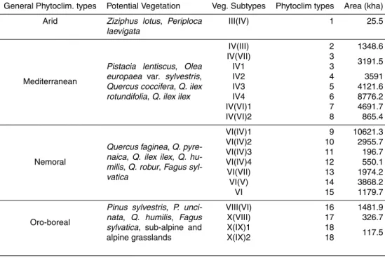
2.2 Phytoclimatic regions

10

The phytoclimatic regions used in this study were delimited according to the classi-fication performed by Allué (1990) in Spain (Table 1), built upon meteorological data from the Spanish Meteorological Agency and the potential vegetation series elabo-rated by Rivas Martínez (1987). The resulting classification consists of 19 di_fferent subtypes of vegetation, each of them linked to characteristic climatic conditions, which 15

are grouped in four general phytoclimatic types, then subdivided into more specific types. Due to the small area encompassed by some of the phytoclimatic zones, we made an aggregation of some of them with the neighbouring units, based on the spatial proximity and ecological affinity in terms of vegetation types. As a result, phytoclimatic types 2–3, 7–8, 10–11–12 and 13–14–15 were merged together for the analyses. In 20

(6)

NHESSD

1, 4891–4924, 2013

burned in Spain

J. Bedia et al.

Title Page

Tables Figures

◭ ◮

Back Close

Full Screen / Esc

Discussion

P

a

per

|

D

iscussion

P

a

per

|

Discussion

P

a

per

|

Discuss

ion

P

a

per

|

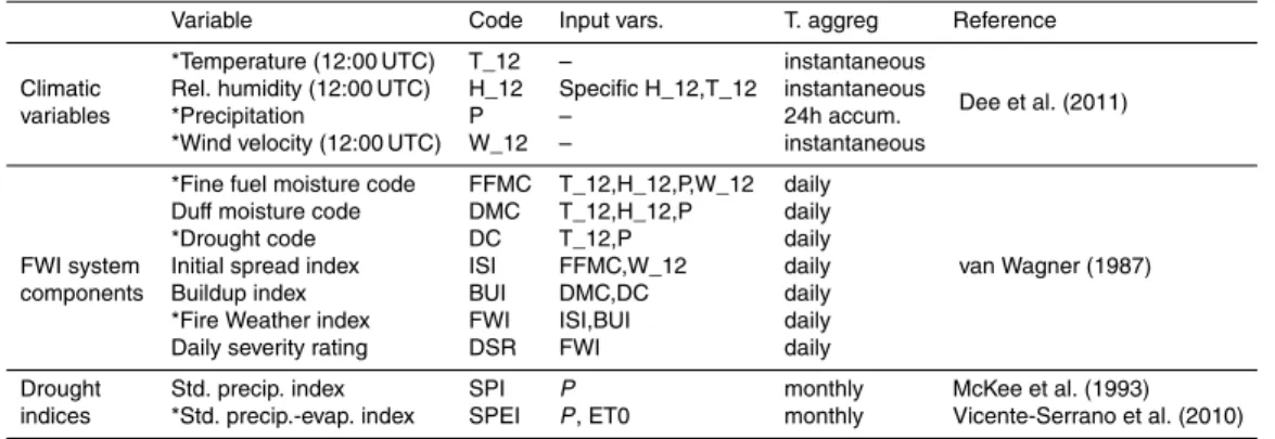
2.3 Climate data

We obtained climate data from the ERA-Interim reanalysis, produced by the Euro-pean Centre for Medium-Range Weather Forecasts in collaboration with many institu-tions (Dee et al., 2011). The performance of di_fferent reanalysis products in the Iberian Peninsula and further details on their use for fire danger estimation are described in 5

(Bedia et al., 2012). The main advantages of reanalysis data are the wide geographi-cal coverage and the homogeneity of the time series provided. In addition, reanalysis products generally provide a large number of variables, including those needed at sur-face level for the reconstruction of FWI series, some of them (in particular wind speed and humidity) difficult to obtain from observational datasets over large areas.

10

2.4 The Canadian Forest Fire Weather Index System

The Fire Weather Index (FWI) System consists of six components rating the e_ffects of fuel moisture content and wind on a daily basis, based on various factors related to potential fire behaviour (van Wagner, 1987; Stocks et al., 1989). The first three components, referred to as the Fine Fuel Moisture Code (FFMC), the Du_ff Moisture 15

Code (DMC) and the Drought Code (DC), rate the average moisture content of diff er-ent soil layers, respectively fine surface litter, decomposing litter, and organic layers. Wind e_ffects are then added to FFMC to form the Initial Spread Index (ISI), which is an indicator of the rate of fire spread. The remaining two fuel moisture codes (DMC and DC) are combined to produce the Build Up Index (BUI), which rates the total amount 20

of fuel available for combustion. BUI is finally combined with ISI to produce the Fire Weather Index (FWI), a dimensionless index rating the potential fire line intensity given the meteorological conditions at noon local standard time in a reference fuel type (ma-ture pine stands). The FWI System uses as input four meteorological variables: daily accumulated precipitation, instantaneous wind speed, instantaneous humidity and in-25

(7)

NHESSD

1, 4891–4924, 2013

burned in Spain

J. Bedia et al.

Title Page

Tables Figures

◭ ◮

Back Close

Full Screen / Esc

Discussion

P

a

per

|

D

iscussion

P

a

per

|

Discussion

P

a

per

|

Discuss

ion

P

a

per

|

2.5 Drought indices

Drought is an important factor related to wildfire occurrence and magnitude (see e.g. Pereira et al., 2005; Littell et al., 2009; Meyn et al., 2010). Unlike the previous daily fire danger indices, droughts are climatic phenomena di_fficult to quantify in terms of inten-sity, magnitude, duration and spatial extent, partly because there is no a straightforward 5

manner to identify their onset, duration and end (Vicente-Serrano et al., 2010). A num-ber of specific indices have been developed in order to quantify and properly describe drought episodes, and in this study we have included two of them: The Standardized Precipitation Index (SPI) and the standardized precipitation-evapotranspiration index (SPEI). Unlike other popular drought indices, both SPI and SPEI account for the widely 10

accepted multi-scalar nature of droughts (see e.g. McKee et al., 1993). Both indices are calculated on a monthly basis, and therefore they have been only tested as predictors in the burned area models.

SPI is an index based on the probability of recording a given amount of precipitation at a specific point and can represent precipitation dynamics over user-selected time 15

frames (McKee et al., 1993). However, SPI does not take into account temperature, and thus may present important deviations from the true water deficits derived from evapotranspiration. As a result, the recently developed SPEI (Vicente-Serrano et al., 2010) was also introduced. In practice, both indices were highly correlated and only SPEI was used for burned area model building (Table 2).

20

2.6 Data Analysis

Climate and fire data were interpolated to a regular grid of 25 km resolution, represent-ing a compromise between the 10 km resolution of the fire information and the≃70 km horizontal resolution of ERA-Interim data. For each pixel, we computed daily time se-ries of climate predictors (except SPEI and SPI, which are monthly, Table 2) and burned 25

(8)

NHESSD

1, 4891–4924, 2013

burned in Spain

J. Bedia et al.

Title Page

Tables Figures

◭ ◮

Back Close

Full Screen / Esc

Discussion

P

a

per

|

D

iscussion

P

a

per

|

Discussion

P

a

per

|

Discuss

ion

P

a

per

|

We tested two different algorithms for model development: generalized linear mod-els (GLM, McCullagh and Nelder, 1989) and multivariate adaptive regression splines (MARS, Friedman, 1991). On the one hand, GLMs constitute a parametric method widely used, thus constituting an adequate benchmarking method. On the other hand, MARS is a non–parametric method for regression. Unlike GLMs, MARS is able to 5

model non-linearities in the data by approximating the underlying function through a set of adaptive piecewise linear regressions – known asbasis functions– of the form:

y=αo+ K X

k=1

αkbk(x), (1)

where the slope of each piecewisebk(x) can change in a set of pointszki,i=1,. . .,mk,

called knots. The popularity of this technique is due to the efficient optimization proce-10

dure used for the iterative search for basis functions and knots.

A comparative study of both MARS and GLM in the context of binary response pre-dictions is done in Bedia et al. (2011, 2013). In both cases, the presence of redundant (highly correlated) predictors may introduce inconsistencies in variable importance es-timates (see Sects. 2.6.1 and 2.6.2). Thus, we first computed the pairwise-correlation 15

matrix with all candidate explanatory variables averaged at the country level, and elim-inated one of each pair attaining correlation coefficients (Spearman’sρ) greater than 0.7. We decided to preserve variable pairs below this threshold in order to avoid the loss of useful information. The resulting subset of explanatory variables is indicated by the asterisks in Table 2.

20

2.6.1 Fire occurrence models

We used generalized linear models (GLM) for fire occurrence model development, con-sidering the logit link function for the binary response variable (fire/no fire), at a daily resolution. We selected GLMs after finding that model performance was similar in this case than with the use of the more sophisticated MARS approach.

(9)

NHESSD

1, 4891–4924, 2013

burned in Spain

J. Bedia et al.

Title Page

Tables Figures

◭ ◮

Back Close

Full Screen / Esc

Discussion

P

a

per

|

D

iscussion

P

a

per

|

Discussion

P

a

per

|

Discuss

ion

P

a

per

|

In order to analyse the effect of spatial aggregation of data in the models, we tested two di_fferent approaches of spatial aggregation of the data:

– Grid-box models: A full matrix of occurrence/absence of fires was constructed for each phytoclimatic zone, considering all the grid-boxes encompassed within the zone and the full daily time series (Fig. 3a). This will be referred to as thegrid-box

5

approach hereafter.

– Areal models: Occurrence/no occurrence data were aggregated at the phytocli-matic zone level, considering as occurrences all days in which at least one fire at one grid box took place, and absences to those days in which no fire took place at any of the grid boxes (Fig. 3c). This will be referred to as theareal approach 10

hereafter.

In order to test the sensitivity of the models to fire size, we set different burned area thresholds for occurrence definition: 0.1, 1, 10 and 100 ha. As a result, only fires above the corresponding area thresholds were computed as occurrences.

Fire occurrence models were trained using all occurrence samples and fire absences 15

randomly chosen in an equal number to the fire occurrences, thus using balanced datasets for model training to avoid an artificial inflation of model skill (see, e.g.: Manel et al., 2001; McPherson et al., 2004). For the grid-box model training, fire absences were sampled only from those days in which no fires occurred in any of the grid-boxes of the phytoclimatic zone (i.e., those rows of matrix in Fig. 3a in which all values are 20

equal to zero), and this process was repeated 100 times in order to get a confidence interval of the sampling error. We then tested the resulting models using a random sample containing all possible cases. We undertook a one-year out cross-validation procedure, using 18 yr for training and the remaining one for testing, repeating this pro-cess 19 times, exactly one per year. From the resulting probabilistic predictions (see 25

(10)

NHESSD

1, 4891–4924, 2013

burned in Spain

J. Bedia et al.

Title Page

Tables Figures

◭ ◮

Back Close

Full Screen / Esc

Discussion

P

a

per

|

D

iscussion

P

a

per

|

Discussion

P

a

per

|

Discuss

ion

P

a

per

|

possible range of RSA is [0,1]. Zero skill is indicated by RSA=0.5, when the ROC lies along the positive diagonal, whereas RSA₌1.0 corresponds to a perfect skill. A RSA value below 0.5 corresponds to a ROC curve below the diagonal, indicating the same level of discrimination capacity as if it were reflected about the diagonal, but wrongly calibrated (Jolli_ffe and Stephenson, 2003). In order to compute the predicted 5

fire frequencies, the probabilistic model predictions were converted into a binary pre-diction using two different approaches for decision threshold determination (both are illustrated in the right hand vertical plots of Fig. 3b and c for the grid-box/areal models):

– A global fixed probability threshold was determined by calculating the likelihood ratio of fire occurrence as given by the observations, and then applied to the full 10

vector of predictions. This approach will be termed asglobal thresholdhereafter.

– A monthly-varying threshold, corresponding to the likelihood ratio of fire occur-rence as given by the observation, conditioned to the month. As a result, 12 dif-ferent decision thresholds were obtained for each month of the year, which were applied to the predictions of the corresponding month to obtain the binary predic-15

tion. This threshold is referred to asmonthly thresholdin the following.

In order to estimate variable importance in the context of logistic regression, we applied the method of hierarchical partitioning, by which the independent e_ffect of each variable is calculated by comparing the fit of all models containing a particular variable to the fit of all nested models lacking that variable (Chevan and Sutherland, 1991). For 20

instance, for variableX₁, its importanceIwould be calculated as follows:

Ix1= k₋1 X

i=0 P

(r_y2_,_X

1Xh−r 2 y,X_h)/

k−1

i

k (2)

whereXhis any subset ofipredictors from whichX1is excluded. As a result, the

(11)

NHESSD

1, 4891–4924, 2013

burned in Spain

J. Bedia et al.

Title Page

Tables Figures

◭ ◮

Back Close

Full Screen / Esc

Discussion

P

a

per

|

D

iscussion

P

a

per

|

Discussion

P

a

per

|

Discuss

ion

P

a

per

|

attributable to each predictor. This method provides a robust assessment of variable importance and has been shown to outperform other methods used for variable impor-tance estimation in the context of regression analysis (Murray and Conner, 2009).

2.6.2 Burned area models

For the burned area models, we aggregated both fire and climate data in a monthly 5

basis (1990–2008,N=228 months). We used MARS as modelling algorithm because it performs well in the presence of outlying observations, as it is the case of large, infrequent fires. For this reason, it has been used in previous studies for modelling burned area (see e.g., Balshi et al., 2009; Amatulli et al., 2013).

In order to obtain robust estimates of model performance, we carried out a Leave-10

One-Out Cross Validation procedure (LOOCV) to compute the error (Michaelsen, 1987). LOOCV is a resampling technique in whichn−1 instances out of the total ofn, are used as the training dataset and the remaining one is used for testing. The procedure is re-peated n times, one per observed instance, producing a more precise estimation of the classification accuracy. The method assumes that each sample is independent, so 15

prior to its application we constructed autocorrelation plots of the monthly burned ar-eas. We found a slight autocorrelation (maximum of 0.26) at some phytoclimatic types that resulted significant at theα=0.05 level. However, time series with autocorrelation of 0.25 or less will have an effective sample size at least of 90 % of the original sample size (Michaelsen, 1987), and thus it can be considered that this does not produce any 20

measurable e_ffect on the LOOCV estimates.

For variable importance estimation in the context of MARS, we looked at the re-ductions in the Generalized Cross–Validation estimate of error (GCV) in the selection routine performed by the MARS algorithm (Kuhn, 2010). The GCV is reduced each time a new variable is entered into the model. The accumulated reductions in GCV 25

(12)

NHESSD

1, 4891–4924, 2013

burned in Spain

J. Bedia et al.

Title Page

Tables Figures

◭ ◮

Back Close

Full Screen / Esc

Discussion

P

a

per

|

D

iscussion

P

a

per

|

Discussion

P

a

per

|

Discuss

ion

P

a

per

|

All the analyses were conducted in the R language and environment for statistical computing (R Core Team, 2013). The hierarchical partitioning was undertaken using theRpackagehier.part (Walsh and Mac Nally, 2013). For the MARS models, we used the implementation of the algorithm included in the R packageearth (Milbor-row, 2013). The drought indices SPI and SPEI were computed using the R package 5

SPEI(Beguería and Vicente-Serrano, 2013).

3 Results and discussion

3.1 Fire regimes of the di_fferent phytoclimatic regions

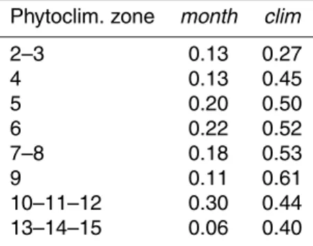
We found two contrasting fire regimes in terms of area burned and number of fires across phytoclimatic zones: one characterized by a bimodal annual pattern, and an-10

other one exhibiting an unimodal annual cycle, with the fire season concentrated in the summer months (Fig. 2). The first case corresponds to the phytoclimatic types un-der the Atlantic influence (10–11–12 and 13–14–15), with two peaks of fire activity in March and August. These regions are characterized by temperate and wet conditions during most of the year, and also by relatively low fire danger conditions. In spite of 15

the less suitable conditions for fire activity of these regions, there is a high number of fire records and also large burned areas. With this regard, previous studies highlight the strong influence that humans exert on fire regimes, and how fire incidence can be greatly enhanced for this reason even when climate conditions are not the most favourable (Vázquez et al., 2002). On the other hand, in the remaining phytoclimatic 20

(13)

NHESSD

1, 4891–4924, 2013

burned in Spain

J. Bedia et al.

Title Page

Tables Figures

◭ ◮

Back Close

Full Screen / Esc

Discussion

P

a

per

|

D

iscussion

P

a

per

|

Discussion

P

a

per

|

Discuss

ion

P

a

per

|

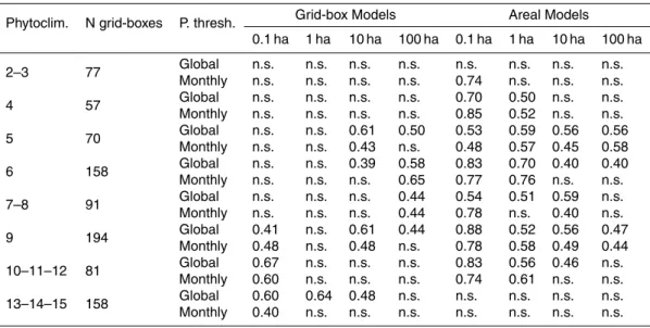
3.2 Fire occurrence model performance and fire frequency results

Most phytoclimatic zones attained good model performance, and only zones 2–3, 10– 11–12 and 13–14–15 yielded RSA values below 0.7 (Table 3). In terms of RSA, the models attained higher skills with increasing burned area thresholds, showing that the fire weather predictors used are more sensitive to the detection of larger fires than to 5

smaller ones, being the latter not so closely dependent on favourable climate conditions for their occurrence. In all cases, the sampling error related to the random selection of days without fires was very low.

However, the good model skills are not directly linked to a good reproducibility of ob-served fire frequencies when working at the grid-box scale. With this regard, all models 10

tended to a large overestimation of fire occurrence at this spatial scale, because all events of high danger potential are given a high probability of occurrence, in close re-lationship with the annual cycle of fire-weather danger (Fig. 3b). However, this effect is overridden when considering a larger spatial aggregation unit, because the probability of having at least one fire in a larger region when the conditions are favourable is much 15

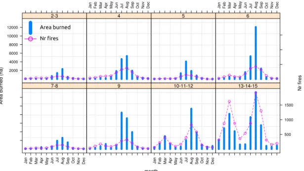
higher. This is illustrated in the observed and predicted fire occurrences/probabilities in Fig. 3c and d, evidencing the adequacy of the phytoclimatic zones defined as spa-tial aggregation units. As a result of areal aggregation, the predicted and observed magnitudes of fire frequencies are directly comparable (Fig. 4), attaining high correla-tion coe_fficients for some phytoclimatic zones (Table 4). Furthermore, the similar fire 20

regimes of some phytoclimatic zones (Fig. 2) suggests the possibility of further aggre-gation into larger spatial units, leaving the door opened to the eventual improvement of model results. In the same vein, due to the marked seasonality of the fire danger potential, the seasonal adjustment of the probability threshold for case classification yielded in most occasions similar or better results than the global probability threshold 25

(e.g. in phytoclimatic zones 2–3, 6, 9, 10–11–12, Table 4 and Fig. 4).

(14)

NHESSD

1, 4891–4924, 2013

burned in Spain

J. Bedia et al.

Title Page

Tables Figures

◭ ◮

Back Close

Full Screen / Esc

Discussion

P

a

per

|

D

iscussion

P

a

per

|

Discussion

P

a

per

|

Discuss

ion

P

a

per

|

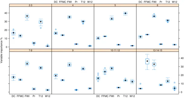
of the FWI system (DC, FFMC). For the sake of conciseness, the results for the occur-rence models are illustrated for the 10 ha burned area threshold models, although very similar results were obtained for the remaining burned area thresholds (Fig. 6).

3.2.1 Burned area models

Burned area was modelled with uneven accuracy depending on the phytoclimatic zone 5

considered. The climatic predictors used as explanatory variables in the models pro-vided an added explained variation when compared against a simple model incor-porating only the annual cycle (respectively denoted as clim and month in Table 6), and therefore the skill of the models can not be solely attributed to the seasonal cy-cle of the fire danger predictors. The best result was attained in phytoclimatic zone 9 10

(R2=0.61). In general terms, our results are comparable to previous analyses per-formed at a similar temporal scale (Amatulli et al., 2013). These authors also found considerable variability in model performance among different European countries, in a similar way as we find them across phytoclimatic regions in Spain. The reasons be-hind the idiosyncratic results of burned area models may lie in the presence of outlying 15

observations (i.e. very large exceptional fires, see e.g. Trigo et al., 2006), and the in-fluence of other landscape and anthropogenic factors beyond the explanatory ability of the climatic drivers in some regions (Viedma et al., 2006; Costa et al., 2011). Similarly, high fire danger situations may not directly translate into large burned areas; for in-stance, burned area may result less predictable in areas with complex topography (Bal-20

shi et al., 2009), such as the northern parts of Spain. Furthermore, the e_ffectiveness of fire suppression schemes may prevent from the occurrence of large fires in situa-tions of high fire danger (see e.g. Turco et al., 2013). Further complicasitua-tions arise from the interpretation of fire history from records of burned area alone (see e.g. Niklasson and Granstrom, 2000). For instance, the same burned area might be the result of a few 25

(15)

NHESSD

1, 4891–4924, 2013

burned in Spain

J. Bedia et al.

Title Page

Tables Figures

◭ ◮

Back Close

Full Screen / Esc

Discussion

P

a

per

|

D

iscussion

P

a

per

|

Discussion

P

a

per

|

Discuss

ion

P

a

per

|

indicated by the lower performance of these models in the Atlantic regions 10–11–12 and 13–14–15 in Table 3 –.

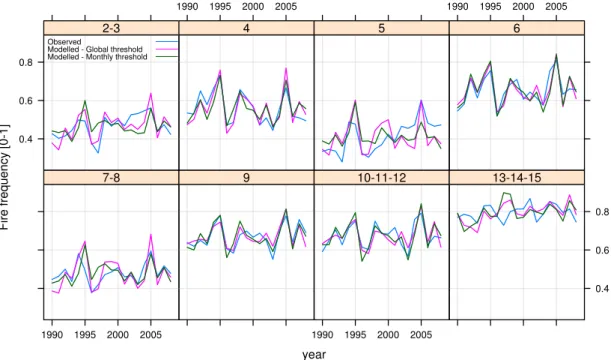
As a result, the predictability of burned area resulted unstable, and in most zones we obtained non-significant inter-annual burned area cross-correlations between ob-served and predicted time series, with the presence of some outlying predictions (as in 5

zone 4, year 1994) and even a spurious negative significant correlation in the case of phytoclimatic zone 2–3 (Fig. 5). Nevertheless, it is remarkable the good reproducibility of annual burned areas attained in phytoclimatic zone 6, and to a lesser extent in zones 9 and 10–11–12, although the results of annual fire frequencies are much more robust and consistent across zones (Table 4).

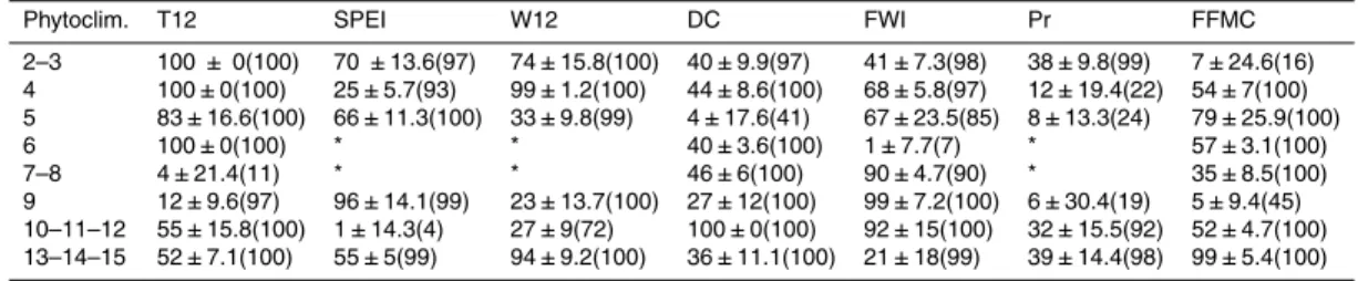
10

Regarding the climatic controls of burned area, the drought index SPEI was an im-portant predictor in some phytoclimatic zones (Table 5), notably in the model of zone 9, which is the one attaining the highest explained variance (Table 6), and also performed well in the representation of annual burned areas (Spearman’s ρ=0.56, Fig. 5). On the contrary, SPEI was not selected by the models in other zones (6, 7–8, 10–11–12), 15

suggesting that the effect of drought on fire size is very different depending on the vege-tation types. Temperature, DC, FWI and FFMC were selected by all models with varying importance, although all models always selected a FWI system component and/or tem-perature as the most important variables, indicating the importance of these predictors at the monthly scale for the estimation of burned area. In the particular case of zone 6 20

– which obtained the highest inter-annual correlation with observed burned area – the most important explanatory variables were temperature, and the FWI components DC and FFMC.

4 Conclusions

Our results support the use of ERA-Interim reanalysis and the FWI system for fire 25

(16)

NHESSD

1, 4891–4924, 2013

burned in Spain

J. Bedia et al.

Title Page

Tables Figures

◭ ◮

Back Close

Full Screen / Esc

Discussion

P

a

per

|

D

iscussion

P

a

per

|

Discussion

P

a

per

|

Discuss

ion

P

a

per

|

good model skill in terms of RSA, although this fact does not translate directly into a good reproducibility of fire frequencies, due to the inherent tendency of the method to over-estimate fire occurrence. Nonetheless, the annual cycle was adequately mod-elled regardless of the distributional characteristics of the different annual fire regimes of each phytoclimatic zone. Temperature and some components of the FWI system 5

(FWI itself and DC and FFMC in particular) were the most important predictors of fire occurrence.

Areal models yielded accurate predictions of the inter-annual fire frequency series, showing that the aggregation of the data into larger spatial units is needed for an ade-quate analysis the climatic drivers of fires, and that the phytoclimatic zones used in this 10

study constitute representative units of the climate-fire relationship, without prejudice to the application of other convenient aggregation units as long as this representative-ness is preserved, such as the different phytoclimatic/bioclimatic classifications avail-able at di_fferent scales throughout the world, or other type of classifications based on fire regime characteristics (see e.g. Archibald et al., 2013).

15

We attained fair burned area model results for some phytoclimatic zones, although most of them failed to adequately reproduce the inter-annual burned area series, with some exceptions. In all cases, burned areas were mostly explained by temperature and drought-related indices bearing some sort of “memory” on the antecedent conditions, such as the FWI system components DC and FFMC, or the recently developed drought 20

index SPEI. As a result, the practical application of burned area models for certain aims, such as the prediction of future burned area scenarios, poses important limitations, being the fire frequency models more robust to this aim.

Acknowledgements. We are grateful to Pilar Martín and Israel Gómez for their help with fire data gathering. The research leading to these results has received funding from the European

25

(17)

NHESSD

1, 4891–4924, 2013

burned in Spain

J. Bedia et al.

Title Page

Tables Figures

◭ ◮

Back Close

Full Screen / Esc

Discussion

P

a

per

|

D

iscussion

P

a

per

|

Discussion

P

a

per

|

Discuss

ion

P

a

per

|

References

Allué, J.: Atlas Fitoclimático de España. Taxonomías, Tech. rep., Instituto Nacional de Investi-gaciones Agrarias, Ministerio de Agricultura, Pesca y Alimentación, Madrid, Spain, 221 pp., 1990. 4894, 4895

Amatulli, G., Camia, A., and San-Miguel-Ayanz, J.: Estimating future burned areas under

5

changing climate in the EU-Mediterranean countries, Sci. Total Environ., 450–451, 209–222, 2013. 4901, 4904

Archibald, S., Lehmann, C. E. R., Gomez-Dans, J. L., and Bradstock, R. A.: Defining pyromes and global syndromes of fire regimes, Proc. Natl. Aca. Sci. USA, 110, 6442–6447, 2013. 4906

10

Balshi, M., McGuire, A., Duffy, P., Flannigan, M., Walsh, J., and Melillo, J.: Assessing the re-sponse of area burned to changing climate in wester boreal North America using a Multi-variate Adaptive Regression Splines (MARS) approach, Global Change Biol., 15, 578–600, 2009. 4901, 4904

Barbati, A., Arianoutsou, M., Corona, P., De Las Heras, J., Fernandes, P., Moreira, F.,

Papageor-15

giou, K., Vallejo, R., and Xanthopoulos, G.: Post-fire forest management in southern Europe: a COST action for gathering and disseminating scientific knowledge, Iforest-Biogeosciences and Forestry, 3, 5–7, 2010. 4893

Bedia, J., Busqué, J., and Gutiérrez, J. M.: Predicting plant species distribution across an alpine rangeland in northern Spain: a comparison of probabilistic methods, Appl. Veg. Sci., 14, 415–

20

432, 2011. 4898

Bedia, J., Herrera, S., Gutiérrez, J. M., Zavala, G., Urbieta, I. R., and Moreno, J. M.: Sensitivity of fire weather index to different reanalysis products in the Iberian Peninsula, Nat. Hazards Earth Syst. Sci., 12, 699–708, doi:10.5194/nhess-12-699-2012, 2012. 4894, 4896

Bedia, J., Herrera, S., and Gutiérrez, J. M.: Dangers of using global bioclimatic datasets for

25

ecological niche modeling. Limitations for future climate projections, Global Planet. Change, 107, 1–12, 2013. 4898

Beerling, D. J. and Osborne, C. P.: The origin of the savanna biome, Global Change Biol., 12, 2023–2031, 2006. 4893

Beguería, S. and Vicente-Serrano, S. M.: SPEI: Calculation of the Standardised

Precipitation-30

(18)

NHESSD

1, 4891–4924, 2013

burned in Spain

J. Bedia et al.

Title Page

Tables Figures

◭ ◮

Back Close

Full Screen / Esc

Discussion

P

a

per

|

D

iscussion

P

a

per

|

Discussion

P

a

per

|

Discuss

ion

P

a

per

|

Bond, W., Woodward, F., and Midgley, G.: The global distribution of ecosystems in a world without fire, New Phytologist, 165, 525–537, 2005. 4893

Bowman, D. M. J. S., Balch, J. K., Artaxo, P., Bond, W. J., Carlson, J. M., Cochrane, M. A., D’Antonio, C. M., DeFries, R. S., Doyle, J. C., Harrison, S. P., Johnston, F. H., Keeley, J. E., Krawchuk, M. A., Kull, C. A., Marston, J. B., Moritz, M. A., Prentice, I. C., Roos, C. I., Scott,

5

A. C., Swetnam, T. W., van der Werf, G. R., and Pyne, S. J.: Fire in the Earth System, Science, 324, 481–484, 2009. 4893

Chevan, A. and Sutherland, M.: Hierarchical Partitioning, The American Statistician, 45, 90–96, 1991. 4900

Costa, L., Thonicke, K., Poulter, B., and Badeck, F.-W.: Sensitivity of Portuguese forest fires

10

to climatic, human, and landscape variables: subnational differences between fire drivers in extreme fire years and decadal averages, Reg. Environ. Change, 11, 543–551, 2011. 4904 Dee, D. P., Uppala, S. M., Simmons, A. J., Berrisford, P., Poli, P., Kobayashi, S., Andrae, U.,

Balmaseda, M. A., Balsamo, G., Bauer, P., Bechtold, P., Beljaars, A. C. M., van de Berg, L., Bidlot, J., Bormann, N., Delsol, C., Dragani, R., Fuentes, M., Geer, A. J., Haimberger,

15

L., Healy, S. B., Hersbach, H., Hólm, E. V., Isaksen, L., Kållberg, P., Köhler, M., Matricardi, M., McNally, A. P., Monge-Sanz, B. M., Morcrette, J., Park, B., Peubey, C., de Rosnay, P., Tavolato, C., Thépaut, J.-N., and Vitart, F.: The ERA-Interim reanalysis: configuration and performance of the data assimilation system, Q. J. R. Meteorol. Soc., 137, 553–597, 2011. 4896, 4913

20

Friedman, J. H.: Multivariate adaptive regression splines, Ann. Stat., 19, 1–67, 1991. 4898 Hardy, C.: Wildland fire hazard and risk: Problems, definitions, and context, FOREST

ECOL-OGY AND MANAGEMENT, 211, 73–82, Symposium on Relative Risk Assessments for Decision-Making Related to Uncharacteristic Wildfire, Portland, OR, NOV, 2003, 2005. 4893 Jolliffe, I. and Stephenson, D. (Eds.): Forecast Verification. A Practitioner’s guide in Atmospheric

25

Science, Wiley, Chichester, England, 2003. 4900

Keeley, J.: Impact of antecedent climate on fire regimes in coastal California, Int. J. Wildland Fire, 13, 173–182, 2004. 4893

Koutsias, N., Arianoutsou, M., Kallimanis, A., Mallinis, G., Halley, J., and P., D.: Where did the fires burn in Peloponnisos, Greece, the summer of 2007? Evidence for a synergy of fuel and

30

(19)

NHESSD

1, 4891–4924, 2013

burned in Spain

J. Bedia et al.

Title Page

Tables Figures

◭ ◮

Back Close

Full Screen / Esc

Discussion

P

a

per

|

D

iscussion

P

a

per

|

Discussion

P

a

per

|

Discuss

ion

P

a

per

|

Kuhn, M.: Variable importance using the caret package, The Comprehensive R Archive Network, available at: http://cran.open-source-solution.org/web/packages/caret/vignettes/ caretVarImp.pdf (last access: 16 September 2013), 2010. 4901

Littell, J., McKenzie, D., Peterson, D., and Westerling, A.: Climate and wildfire area burned in western U.S. ecoprovinces, 1916–2003, Ecol. Appl., 19, 1003–1021, 2009. 4897

5

Manel, S., Williams, H. C., and Ormerod, S. J.: Evaluating presence-absence models in ecol-ogy: the need to account for prevalence, J. Appl. Ecol., 38, 921–931, 2001. 4899

Marlon, J. R., Bartlein, P. J., Carcaillet, C., Gavin, D. G., Harrison, S. P., Higuera, P. E., Joos, F., Power, M. J., and Prentice, I. C.: Climate and human influences on global biomass burning over the past two millennia, Nat. Geosci., 1, 697–702, 2008. 4893

10

McCullagh, P. and Nelder, J.: Generalized linear models, Chapman & Hall, London, 1989. 4898 McKee, T., Doesken, J., and Kleist, J.: The relationship of drought frecuency and duration to time scales, in: Proceedings of the Eight Conf. On Applied Climatology, Anaheim, CA, Amer-ican Meteorological Society, 179–184, 1993. 4897, 4913

McPherson, J., Jetz, W., and Rogers, D.: The effects of species’ range sizes on the accuracy of

15

distribution models: ecological phenomenon or statistical artefact?, J. Appl. Ecol., 41, 811– 823, 2004. 4899

Mérida, J., Primo, E., Eleazar, J., and Parra, J.: Las Bases de Datos de Incendios Fore-stales como herramienta de planificación: utilización en España por el Ministerio de Medio Ambiente, in: Proceedings of the 4th International Wildland Fire Conference,

20

Sevilla, Spain, 13–18 May 2007, edited by: Organismo Autónomo de Parques Nacionales, M. d. M. A., available at: http://www.fire.uni-freiburg.de/sevilla-2007/contributions/doc/ cd/SESIONES_TEMATICAS/ST4/Merida_et_al_SPAIN_DGB.pdf (last access: 9 Septem-ber 2013), 2007 (in Spanish). 4895

Meyn, A., White, P. S., Buhk, C., and Jentsch, A.: Environmental drivers of large, infrequent

25

wildfires: the emerging conceptual model, Prog. Phys. Geogr., 31, 287–312, 2007. 4894 Meyn, A., Schmidtlein, S., Taylor, S., Girardin, M., Thonicke, K., and Cramer, W.: Spatial

varia-tion of trends in wildfire and summer drought in British Columbia, Canada, 1920–2000, Int. J. Wildland Fire, 19, 272–283, 2010. 4897

Michaelsen, J.: Cross-Validation in Statistical Climate Forecast Models, J. Clim. Appl. Meteorol.,

30

(20)

NHESSD

1, 4891–4924, 2013

burned in Spain

J. Bedia et al.

Title Page

Tables Figures

◭ ◮

Back Close

Full Screen / Esc

Discussion

P

a

per

|

D

iscussion

P

a

per

|

Discussion

P

a

per

|

Discuss

ion

P

a

per

|

Milborrow, S.: earth: Multivariate Adaptive Regression Spline Models, available at: http://CRAN. R-project.org/package=eart (last access: 16 September 2013), R package version 3.2-6, 2013. 4902

Murray, K. and Conner, M.: Methods to quantify variable importance: implications for the anal-ysis of noisy ecological data, Ecology, 90, 348–355, 2009. 4901

5

Niklasson, M. and Granstrom, A.: Numbers and sizes of fires: Long-term spatially explicit fire history in a Swedish boreal landscape, Ecology, 81, 1484–1499, 2000. 4904

Pausas, J.: Changes in fire and climate in the Eastern Iberian Peninsula (Mediterranean Basin), Climatic Change, 63, 337–350, 2004. 4893

Pausas, J. G. and Paula, S.: Fuel shapes the fire-climate relationship: evidence from

Mediter-10

ranean ecosystems, Global Ecol. Biogeogr., 21, 1074–1082, 2012. 4893

Pereira, M., Trigo, R., da Camara, C., Pereira, J., and Leite, S.: Synoptic patterns associated with large summer forest fires in Portugal, Agr. Forest Meteorol., 129, 11–25, 2005. 4893, 4897

R Core Team: R: A Language and Environment for Statistical Computing, R Foundation for

15

Statistical Computing, Vienna, Austria, available at: http://www.R-project.org/ (16 Septem-ber 2013), 2013. 4902

Rivas Martínez, S.: Mapa de las Series de Vegetación de la Península Ibérica, Tech. rep., ICONA. Ministerio de Agricultura, Pesca y Alimentación, 1987. 4895

Stocks, B., Lawson, B., Alexander, M., Van Wagner, C., McAlpine, R., Lynham, T., and Dube,

20

D.: The Canadian Forest Fire Danger Rating System – An Overview, For. Chron., 65, 450– 457, 1989. 4896

Swets, J.: Measuring the accuracy of diagnostic systems, Science, 240, 1285–1293, 1988. 4899

Trigo, R., Pereira, J., Pereira, M., Mota, B., Calado, T., DaCamara, C., and Santo, F.:

Atmo-25

spheric conditions associated with the exceptional fire season of 2003 in Portugal, Int. J. Climatol., 26, 1741–1757, 2006. 4904

Turco, M., Llasat, M., von Hardenberg, J., and Provenzale, A.: Impact of climate variability on summer fires in a Mediterranean environment (northeastern Iberian Peninsula), Climatic Change, 116, 665–678, doi:10.1007/s10584-012-0505-6, 2012. 4893

30

(21)

NHESSD

1, 4891–4924, 2013

burned in Spain

J. Bedia et al.

Title Page

Tables Figures

◭ ◮

Back Close

Full Screen / Esc

Discussion

P

a

per

|

D

iscussion

P

a

per

|

Discussion

P

a

per

|

Discuss

ion

P

a

per

|

van Wagner, C. E.: Development and structure of the Canadian Forest Fire Weather Index, Forestry Tech. Rep. 35, Canadian Forestry Service, Ottawa, Canada, 1987. 4896, 4913 Vázquez, A., Pérez, B., Fernández-González, F., and Moreno, J.: Recent fire regime

character-istics and potential natural vegetation relationships in Spain, J. Veg. Sci., 13, 663–676, 2002. 4902

5

Vicente-Serrano, S., Beguería, S., and López-Moreno, J.: A Multi-scalar drought index sensi-tive to global warming: The Standardized Precipitation Evapotranspiration Index – SPEI, J. Climate, 7, 1696–1718, doi:10.1175/2009JCLI2909.1, 2010. 4897, 4913

Viedma, O., Moreno, J. M., and Rieiro, I.: Interactions between land use/land cover change, for-est fires and landscape structure in Sierra de Gredos (Central Spain), Environ. Conservation,

10

33, 212–222, 2006. 4904

(22)

NHESSD

1, 4891–4924, 2013

burned in Spain

J. Bedia et al.

Title Page

Tables Figures

◭ ◮

Back Close

Full Screen / Esc

Discussion

P

a

per

|

D

iscussion

P

a

per

|

Discussion

P

a

per

|

Discuss

ion

P

a

per

|

Table 1.The spatial distribution of the phytoclimatic types is displayed in Fig. 1. Note that the

area is referred to each phytoclimatic type.

General Phytoclim. types Potential Vegetation Veg. Subtypes Phytoclim types Area (kha)

Arid Ziziphus lotus, Periploca laevigata

III(IV) 1 25.5

Mediterranean

Pistacia lentiscus, Olea europaea var. sylvestris, Quercus coccifera,Q. ilex rotundifolia,Q. ilex ilex

IV(III) 2 1348.6

IV(VII) 3

3191.5

IV1 3

IV2 4 3591

IV3 5 4121.6

IV4 6 8776.2

IV(VI)1 7 4691.7

IV(VI)2 8 865.4

Nemoral

Quercus faginea,Q. pyre-naica,Q. ilex ilex,Q. hu-milis,Q. robur,Fagus syl-vatica

VI(IV)1 9 10621.3

VI(IV)2 10 2955.7

VI(IV)3 11 196.7

VI(IV)4 12 550.1

VI(VII) 13 1974.2

VI(V) 14 3868.2

VI 15 1179.7

Oro-boreal

Pinus sylvestris, P. unci-nata, Q. humilis, Fagus sylvatica, sub-alpine and alpine grasslands

VIII(VI) 16 1481.9

X(VIII) 17 326.7

X(IX)1 18

117.5

(23)

NHESSD

1, 4891–4924, 2013

burned in Spain

J. Bedia et al.

Title Page

Tables Figures

◭ ◮

Back Close

Full Screen / Esc

Discussion

P

a

per

|

D

iscussion

P

a

per

|

Discussion

P

a

per

|

Discuss

ion

P

a

per

|

Table 2.Summary of predictors tested in this study for fire model building. After checking for

redundancy, a final subset of weakly-correlated variables was used for model building, marked with an asterisk (Note that SPEI is a monthly indicator, and therefore it was only used as predictor for the burned area models). [ET0=potential evapotranspiration].

Variable Code Input vars. T. aggreg Reference *Temperature (12:00 UTC) T_12 – instantaneous

Dee et al. (2011) Climatic Rel. humidity (12:00 UTC) H_12 Specific H_12,T_12 instantaneous

variables *Precipitation P – 24h accum. *Wind velocity (12:00 UTC) W_12 – instantaneous *Fine fuel moisture code FFMC T_12,H_12,P,W_12 daily

van Wagner (1987) Duffmoisture code DMC T_12,H_12,P daily

*Drought code DC T_12,P daily FWI system Initial spread index ISI FFMC,W_12 daily components Buildup index BUI DMC,DC daily *Fire Weather index FWI ISI,BUI daily Daily severity rating DSR FWI daily

(24)

NHESSD

1, 4891–4924, 2013

burned in Spain

J. Bedia et al.

Title Page

Tables Figures

◭ ◮

Back Close

Full Screen / Esc

Discussion

P

a

per

|

D

iscussion

P

a

per

|

Discussion

P

a

per

|

Discuss

ion

P

a

per

|

Table 3.ROC skill area (RSA) attained by the fire occurrence models for each phytoclimatic

zone. The quantilic range (97.5–2.5 %) after 100 randomly selected fire absences is indicated in parenthesis. Results are presented for the different burned area thresholds used for fire occurrence definition.

Phyt. zone 0.1 ha 1 ha 10 ha 100 ha 2–3 0.67(0.01) 0.68(0.02) 0.73(0.04) 0.77(0.10)

(25)

NHESSD

1, 4891–4924, 2013

burned in Spain

J. Bedia et al.

Title Page

Tables Figures

◭ ◮

Back Close

Full Screen / Esc

Discussion

P

a

per

|

D

iscussion

P

a

per

|

Discussion

P

a

per

|

Discuss

ion

P

a

per

|

Table 4.Spearman’sρcross–correlation coefficients between the observed and predicted

an-nual fire frequencies, determined using the global and monthly probability thresholds. The re-sults correspond to both the the grid-box and areal models. The number of grid-boxes com-prising each phytoclimatic zone are indicated by theN grid-boxescolumn (see the legend of Fig. 1 for a visual indication of their size). The results are presented for the different burned area thresholds used to define fire occurrence/absence. n.s. indicates that the correlation was not significant at the 95 % confidence interval.

Phytoclim. N grid-boxes P. thresh. Grid-box Models Areal Models 0.1 ha 1 ha 10 ha 100 ha 0.1 ha 1 ha 10 ha 100 ha

2–3 77 Global n.s. n.s. n.s. n.s. n.s. n.s. n.s. n.s. Monthly n.s. n.s. n.s. n.s. 0.74 n.s. n.s. n.s.

4 57 Global n.s. n.s. n.s. n.s. 0.70 0.50 n.s. n.s. Monthly n.s. n.s. n.s. n.s. 0.85 0.52 n.s. n.s.

5 70 Global n.s. n.s. 0.61 0.50 0.53 0.59 0.56 0.56 Monthly n.s. n.s. 0.43 n.s. 0.48 0.57 0.45 0.58

6 158 Global n.s. n.s. 0.39 0.58 0.83 0.70 0.40 0.40 Monthly n.s. n.s. n.s. 0.65 0.77 0.76 n.s. n.s.

7–8 91 Global n.s. n.s. n.s. 0.44 0.54 0.51 0.59 n.s. Monthly n.s. n.s. n.s. 0.44 0.78 n.s. 0.40 n.s.

9 194 Global 0.41 n.s. 0.61 0.44 0.88 0.52 0.56 0.47 Monthly 0.48 n.s. 0.48 n.s. 0.78 0.58 0.49 0.44

10–11–12 81 Global 0.67 n.s. n.s. n.s. 0.83 0.56 0.46 n.s. Monthly 0.60 n.s. n.s. n.s. 0.74 0.61 n.s. n.s.

(26)

NHESSD

1, 4891–4924, 2013

burned in Spain

J. Bedia et al.

Title Page

Tables Figures

◭ ◮

Back Close

Full Screen / Esc

Discussion

P

a

per

|

D

iscussion

P

a

per

|

Discussion

P

a

per

|

Discuss

ion

P

a

per

|

Table 5.Variable importance (GCV, in %) of each input variable ± standard deviation, (n=

228 LOOCV models). The percentage of LOOCV models including the variable is indicated in parenthesis. Variables not selected by the MARS algorithm are indicated by asterisks. Note that SPEI is not a candidate variable in the fire occurrence models.

Phytoclim. T12 SPEI W12 DC FWI Pr FFMC 2–3 100 ±0(100) 70±13.6(97) 74±15.8(100) 40±9.9(97) 41±7.3(98) 38±9.8(99) 7±24.6(16) 4 100±0(100) 25±5.7(93) 99±1.2(100) 44±8.6(100) 68±5.8(97) 12±19.4(22) 54±7(100) 5 83±16.6(100) 66±11.3(100) 33±9.8(99) 4±17.6(41) 67±23.5(85) 8±13.3(24) 79±25.9(100) 6 100±0(100) * * 40±3.6(100) 1±7.7(7) * 57±3.1(100) 7–8 4±21.4(11) * * 46±6(100) 90±4.7(90) * 35±8.5(100)

(27)

NHESSD

1, 4891–4924, 2013

burned in Spain

J. Bedia et al.

Title Page

Tables Figures

◭ ◮

Back Close

Full Screen / Esc

Discussion

P

a

per

|

D

iscussion

P

a

per

|

Discussion

P

a

per

|

Discuss

ion

P

a

per

|

Table 6.Explained variance (adjusted-R2, observedvs.predicted) of the LOOCV models for

area burned. The models including only the seasonal cycle (i.e. the month as the only explana-tory variable) are indicated as month. The models using the climatic explanatory variables (Table 2) are indicated asclim.

Phytoclim. zone month clim

2–3 0.13 0.27

4 0.13 0.45

5 0.20 0.50

6 0.22 0.52

7–8 0.18 0.53

9 0.11 0.61

(28)

NHESSD

1, 4891–4924, 2013

burned in Spain

J. Bedia et al.

Title Page

Tables Figures

◭ ◮

Back Close

Full Screen / Esc

Discussion

P

a

per

|

D

iscussion

P

a

per

|

Discussion

P

a

per

|

Discuss

ion

P

a

per

|

2-3 4 5 6 7-8 9 10-11-12 13-14-15

20°W 0° 20°E 40°E 60°E

30

°

N

40

°

N

50

°

N

6

0

°

N

Grid-box size (25km) Phytoclimatic zones

36 38 40 42

-5 0

Fig. 1.Location of the study area. Colour divisions correspond to the different phytoclimatic

(29)

NHESSD

1, 4891–4924, 2013

burned in Spain

J. Bedia et al.

Title Page

Tables Figures

◭ ◮

Back Close

Full Screen / Esc

Discussion

P

a

per

|

D

iscussion

P

a

per

|

Discussion

P

a

per

|

Discuss

ion

P

a

per

|

month

Area

Burned

(ha

)

2000 4000 6000 8000 10000 12000

2-3

Jan Feb Mar Apr May Jun Jul Aug Sep Oct Nov Dec

4 5

Jan Feb Mar Apr May Jun Jul Aug Sep Oct Nov Dec

6

Jan Feb Mar Apr May Jun Jul _Aug _Sep Oct Nov Dec

7-8 9

Jan Feb Mar Apr May Jun Jul _Aug _Sep Oct Nov Dec

10-11-12

500 1000 1500

13-14-15

N

r

fires

Area burned

Nr Þres

Fig. 2.Mean monthly area burned (vertical bars, mainy axis) and mean number of fires (lines

(30)

NHESSD

1, 4891–4924, 2013

burned in Spain

J. Bedia et al.

Title Page

Tables Figures

◭ ◮

Back Close

Full Screen / Esc

Discussion

P

a

per

|

D

iscussion

P

a

per

|

Discussion

P

a

per

|

Discuss

ion

P

a

per

|

(a) (b) (c) (d)

Ti

m

e (N

=

6

94

0 d

ay

(31)

NHESSD

1, 4891–4924, 2013

burned in Spain

J. Bedia et al.

Title Page

Tables Figures

◭ ◮

Back Close

Full Screen / Esc

Discussion

P

a

per

|

D

iscussion

P

a

per

|

Discussion

P

a

per

|

Discuss

ion

P

a

per

|

Fig. 3. Observed and predicted data representation of fire occurrence considering both the

(32)

NHESSD

1, 4891–4924, 2013

burned in Spain

J. Bedia et al.

Title Page

Tables Figures

◭ ◮

Back Close

Full Screen / Esc

Discussion

P

a

per

|

D

iscussion

P

a

per

|

Discussion

P

a

per

|

Discuss

ion

P

a

per

|

year

F

ire

frequency

[0

-1] _0.4 0.6 0.8

2-3

1990 1995 2000 2005

4 5

1990 1995 2000 2005

6

1990 1995 2000 2005

7-8 9

1990 1995 2000 2005 10-11-12

0.4 0.6 0.8 13-14-15

Observed

Modelled - Global threshold Modelled - Monthly threshold

Fig. 4.Observed and 1-year-out cross-validated predicted annual fire frequencies at each

(33)

NHESSD

1, 4891–4924, 2013

burned in Spain

J. Bedia et al.

Title Page

Tables Figures

◭ ◮

Back Close

Full Screen / Esc

Discussion

P

a

per

|

D

iscussion

P

a

per

|

Discussion

P

a

per

|

Discuss

ion

P

a

per

|

year

Burned

area

(l

o

g-transform

ed)

10 15

2-3

1990 1995 2000 2005

4 5

1990 1995 2000 2005

6

1990 1995 2000 2005

7-8 9

1990 1995 2000 2005 10-11-12

10 15 13-14-15

Observed

Modelled rho = n.s. rho = n.s. rho = 0.71

rho = 0.56

rho = n.s. rho = 0.58 rho = n.s.

rho = -0.51

Fig. 5. Observed and cross-validated predicted annual burned areas at each phytoclimatic

(34)

NHESSD

1, 4891–4924, 2013

burned in Spain

J. Bedia et al.

Title Page

Tables Figures

◭ ◮

Back Close

Full Screen / Esc

Discussion

P

a

per

|

D

iscussion

P

a

per

|

Discussion

P

a

per

|

Discuss

ion

P

a

per

|

Vari

able importanc

e %

0 10 20 30 40

2-3

DC FFMC FWI Pr T12 W12

4 5

6

7-8 9

10-11-12

0 10 20 30 40

13-14-15

Fig. 6.Boxplots of variable importance (% of total explained variance) in the fire occurrence