Article
J. Braz. Chem. Soc., Vol. 26, No. 3, 619-631, 2015. Printed in Brazil - ©2015 Sociedade Brasileira de Química 0103 - 5053 $6.00+0.00
A
*e-mail: [email protected]
QSAR Study of the Inhibitors of the Acetyl-CoA Carboxylase 1 and 2 using
Bayesian Regularized Genetic Neural Networks: A Comparative Study
Abolfazl Valadkhani,*,a Mohammad Asadollahi-Babolib and Ahmad Mani-Varnosfaderanic
aDepartment of Analytical Chemistry, Chemistry and Chemical Engineering Research Center of
Iran, Tehran, Iran
bDepartment of Science, Babol University of Technology, Babol, Iran
cDepartment of Chemistry, Tarbiat Modares University, Tehran, Iran
Linear and non-linear quantitative structure-activity relationship (QSAR) models were presented for modeling and predicting anti-diabetic activities of a set of inhibitors of acetyl-CoA carboxylase 1 and 2 (ACC1 and ACC2). Different algorithms were utilized to choose the best variables among large numbers of descriptors and then these selected descriptors were used for non-linear (artificial neural network) and linear (multiple linear regression) modeling. The variable selection methods were consisted of stepwise-multiple linear regression (stepwise-MLR), successive projections algorithm (SPA), genetic algorithm-multiple linear regression (GA-MLR) and Bayesian regularized genetic neural networks (BRGNNs). The prediction abilities of the models were evaluated by Monte Carlo cross validation (MCCV) in variable selection and modeling steps. The results revealed that the best variables for describing the inhibition mechanism of ACC were among topological charge indices, radial distribution function, geometrical, and autocorrelation descriptors. The statistical parameters of R2 and root mean square error (RMSE) indicated that BRGNNs is superior for modeling the
inhibitory activity of ACC modulators over the other methods. The sensitivity analysis together with the frequency of the selected molecular descriptors in this work can establish an understanding to the mechanism of ACC inhibitory activity of small molecules.
Keywords: acetyl-CoA carboxylase, quantitative structure activity relationships, Bayesian regularized genetic neural networks, successive projection algorithm
Introduction
Diabetes mellitus is a typical metabolic disorder characterized by abnormally high levels of plasma glucose or hyperglycemia.1 This disease has been described as
an “epidemic” of contemporary society and threatens to become a global health scourge. The total number of people with diabetes is projected to rise from 171 million in 2000 to 366 million in 2030.2 Furthermore, the World
Health Organization (WHO) estimates that the diabetes deaths account for 5% of global deaths and are likely to expand by more than 50% in the next 10 years without urgent action.3 Mainly two distinct clinical forms of the
diabetes are recognized: the type 1 or insulin-dependent diabetes which is usually diagnosed in the children and young adolescent and is caused by destruction of insulin-producing beta cells in the pancreas, leading to a deficiency
of insulin; type 2 or no-insulin dependent diabetes which is the most common form of diabetes mellitus and is caused by target cell resistance to insulin.
Many recent studies have demonstrated that the obesity is one of the most important risk factors for the prevention of type 2 diabetes and its related co-morbid conditions.4 In
obese individuals, adipose tissue releases increased amounts of non-esterified fatty acids, glycerols, hormones, pro-inflammatory cytokines and other factors that are involved in the development of insulin resistance.5 A drug agent that
purpose is the synthesis of malonyl-CoA (m-CoA) from acetyl-CoA in an ATP-dependent reaction via the fixation of biocarbonate.6 Inhibition of ACC offers the ability to
inhibit de novo fatty acid production in lipogenic tissues (liver and adipose) while at the same time stimulates fatty acid oxidation tissues (heart and skeletal muscle) where it plays a role in modulating energy expenditure.7 Therefore, an
ACC1/2 isozyme nonselective inhibitor would be predicted to reduce fatty acid synthesis in liver and adipose tissue while at the same time increasing fatty acid oxidation in the liver and muscle tissues resulting in increased energy expenditure. The ACC1 and ACC2 enzymes are two important targets in modern drug discovery projects.8 Designing effective
dual ACC1 and ACC2 inhibitors is of great importance for increasing insulin sensitivity and treatment of metabolite syndrome and type 2 diabetes mellitus.9
Recently, 10 screening Pfizer’s compound library
resulted in the identification of a total 60 ACC inhibitors that exhibited good rat and human pharmacokinetics. To discover and design new and more effective compounds, it is necessary to make use of computational techniques and QSAR methods. Thus, the activities of newly designed drugs could be predicted before making a decision whether these compounds should be really synthesized or tested. The construction of a QSAR model often entails the problem of selecting the most relevant predictors from the overall set of predictors. Effective variable selection, therefore, is an integral part of the QSAR modeling process. In the present contribution, four different variable selection techniques followed by neural network modeling have been used for describing and predicting the ACC1 and ACC2 inhibitory activities of a series of arylquinoline amide derivatives. We explored variable selection techniques such as stepwise-multiple linear regression (stepwise-MLR), successive projection algorithm (SPA), genetic-algorithm multiple linear regression (GA-MLR) and Bayesian regularized genetic neural networks (BRGNN). In each of these four methods sampling was done by the use of shuffling on the raw data. In order to deal with the overfitting in both variable selection and modeling procedure, Monte Carlo cross validation (MCCV) and Bayesian regularization formalism (during the training procedure) was used, respectively. The detailed theory behind artificial neural network (ANN) and Bayesian regularization algorithm can be found in literature.11 Section 2 devotes to description of variable
selection, sensitivity analysis and MCCV algorithms. The prediction abilities of the corresponding modeling algorithms will be reported in result and discussion section and the overall results of the various techniques will be compared with each other. This paper help to have a clue
about inhibition mechanism of ACC1 and ACC2 inhibitors and designing new molecules as potent energy modulators for treatment of diabetes mellitus type 2 and metabolite syndrome. The selected molecular descriptors in this work can be considered as informative markers for defining new molecular scaffold with potent ACC inhibitory activities.
Methodology
Variable selection
To build a good QSAR model, a minimal set of information-rich descriptors is required. The large number of possible indices creates several problems for the modeling procedure such as: (a) multicollinearity; (b) poor models generated from poor descriptors; (c) overfitting of the model; (d) lack of relevant molecular information from all of the descriptors (some variables may be irrelevant or unreliable); (e) chance correlation.12 Consequently,
selecting the best descriptors from a large set of variables is crucial for improving the model performance and making better predictions. Many different types of variable selection methods are well known and fully described in the literature.13 In present article, four currently ones are briefly
described, used and compared with each other.
Stepwise multiple linear regression (stepwise-MLR)
A detailed description of the stepwise regression can be found in literature.14 As a short definition, the stepwise
regression method is an iterative selection procedure that starts from a variable with largest empirical correlation with the dependent variable. Each iteration includes two phases: the inclusion phase, in which each of the remaining variables is subjected to a partial F-test. If the largest F-value is larger than a critical “F-to-enter” value, the corresponding variable is inserted in the model. While in the exclusion phase, in which each of the variables is subjected to a partial F-test, if the smallest F-value is smaller than a critical ‘F-to-remove’ value, the corresponding variable will be removed from the model and returned to the pool of variables still available for selection.15
Successive projection algorithm (SPA)
to a criterion that evaluates the prediction ability of the resulting MLR model. Finally in the last phase, the selected subset will undergo an elimination procedure to determine whether any variables can be removed without significant loss of prediction ability. More detail on the successive projections algorithm can be found elsewhere.15
Genetic algorithm-multiple linear regression (GA-MLR)
A genetic algorithm is a simulated technique somewhat inspired by the evolution theory presented by Darwin. Several authors have published papers about feature selection by GAs which can be found in literatures.13,15,16
Briefly, the GA is made up by the following basic steps: (1) a vector (chromosome) containing zeros and ones (genes) is generated with the size corresponding to the number of variables; (2) an initial population of chromosomes is randomly created; (3) the value of fitness function (here MLR and ANN models) is evaluated for each new produced chromosomes; (4) the chromosomes with the best predictions (according to their fitness function value) are used to produce new populations by operations such as selection, crossover and mutation. The fitness function here is the root mean square error of the inhibitory activities calculated by MLR and ANN methods.
Bayesian regularized genetic neural networks (BRGNN)
BRGNN is another combination of genetic algorithms that is utilized for feature selection. This method has been used by Fernández and co-workers17-24 for modeling of
enzyme inhibitors, calcium entry blockers and protein conformational stability.17-24 In BRGNN approach the error
function of Bayesian regularized artificial neural networks (BRANN) is being used as objective function in genetic algorithm for optimization. Actually, each time that GA produces a new population, the created chromosomes serve as inputs to ANN and would be related to the biological activities by the mean of determining the weights and biases in the BRANN model. Thus, GA finds the best chromosomes in order to minimize the residual error between true inhibitory activity values and their calculated quantities. It will be shown that this variable selection method performs more desirable than the others, since it selects the descriptors based on their better correlation with dependent variables in a non-linear manner.
Monte Carlo cross-validation
In order to assess the utility of the model, an estimated model must then be validated. One of the most effective
methods in this case is Monte Carlo cross-validation. By definition, this technique involves a large number of random splits of the dataset repeatedly, in each of which the available data are divided into two groups to be used for the fitting and testing. The criterion, e.g. root mean square error, is averaged over all repeated splits, so as to not tie the measure to one particular division of the data. Moreover, it is essential that the repeats in this modeling exercise incorporate all steps involved in the modeling process, including both feature selection and modeling development.25,26
Sensitivity analysis
There have been a lot of attempts to extract meaning from neural network models because of their complicated structure. Interpretation of ANN can be considered in broad and detailed forms. Broad interpretation characterizes how important an input neuron is to the predictive ability of the model and therefore ranks the input descriptors in order of importance, while the aim of detailed interpretation is to extract the structure-activity trends in an ANN model to indicate how an input descriptor correlates to its corresponding predicted value. Broad interpretation is essentially a “sensitivity analysis” of the neural networks. In this case Guha and Jurs27 have presented a method to measure
the importance property of the descriptor in QSAR model.
Data set
The dataset consists of 60 molecules of arylquinoline amide derivatives together with their inhibitory activities which was gathered from a recently published article by Corbett et al. in 2010.10 In this work, both ACC1 and
ACC2 inhibitory activities were considered as dependent variable for the modeling. The activities involve IC50 and
ligand efficiency (LE) values for rat ACC1 (rACC1) and also IC50 values for human ACC2 (hACC2) inhibitors. The
IC50 values of rACC1 and hACC2 inhibitors were converted
to the logarithmic scale (pIC50). The LE values of rACC1
inhibitors together with the pIC50 values of hACC2 and
rACC1 inhibitors were then used as dependent variables, in our QSAR study. The main skeleton of arylquinoline analogues are given in Figure 1 and the list of the inhibitory activities are displayed in Table 1. Prior to the calculation of the descriptors, the studied compounds were geometrically optimized using semi-empirical AM1 method implemented in Hyperchem software.28 The 3-dimensional structure of
the molecules was encoded to a diverse set of molecular descriptors (up to 1497) using Dragon software.29 The first
values and also descriptors with correlation coefficients higher than 90% were removed from the whole set of independent variables. Thus, the data set consisting of 60 compounds and 657 descriptors was prepared and used for further analysis.
Different variable selection techniques and BRANN modeling
Four different variable selection algorithms were utilized to choose the best variables among the large number of descriptors and then these selected descriptors were used for modeling using BRANN approach. The corresponding m-files of the algorithms were prepared and run in MATLAB software, version R2010a 30 and in each
of these methods, in order to deal with overfitting on both variable selection and modeling procedures, Monte Carlo cross validation and Bayesian regularization formalism were used, respectively. The “neural network” and “global optimization” toolboxes in MATLAB have been used for running BRANN and GA, respectively. The specification of the parameters of GA and BRANN applied for optimization are given in Table S1 in supplementary material section. In order to run the BRGNN algorithm, the BRANN models must be stable inside the GA paradigm. The stability of the BRANN during the GA procedure has been investigated in our previous works.11,31 Similar to our previous works, we
observed a thorough reproducibility with near zero standard deviations in BRANN models in present study.
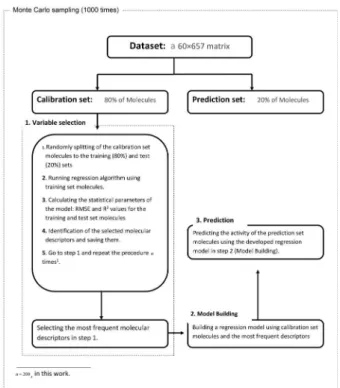
Figure 2 shows a flowchart of the overall algorithm of feature selection and modeling process in this work. It begins by first splitting of the dataset randomly into two parts of prediction set (20% of the raw data) and calibration set (the remaining 80% of the raw data). This procedure repeats for 1000 times. The variable selection on the calibration set, again, repeats for 200 times. In each
variable selection step, the calibration set is randomly divided into two subsets (80% training set and 20% test set), thus leading to the removal of overfitting with a high probability. By the mean of this sampling algorithm, the best and most frequent variables would be chosen. In each run of 1000 runs, after finishing repeating variable selection 200 times, the prediction set with the best selected variables would be applied to the regression algorithm as inputs to fit and evaluate the model’s prediction ability, and then the algorithm continues this procedure until 1000 runs are completed.
It must be noticed that in the case of GA-MLR and BRGNN feature selection methods, the algorithm was defined such as to save and consider the chromosomes of hundreds of the last generations out of 200 generations in each GA run instead of running only the last chromosome. By running this GA variable selection method, adequate information was available to select the best variables among the whole pool of them. Moreover, this makes confidence that the selected variables include all essential descriptors for modeling with regression model and no important variable is missed.
Calculation of the importance of molecular descriptors
According to Guha and Jurs,27 an algorithm was
developed for sensitivity analysis of the constructed ANN
Figure 2. The flowchart of the Monte Carlo sampling and modeling procedure used in the present contribution.
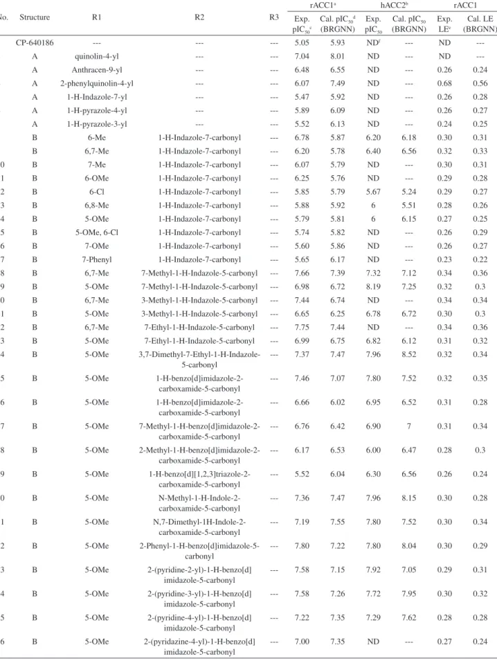
Table 1. The structural information of the ACC inhibitors together with the experimental and calculated pIC50 values
No. Structure R1 R2 R3
rACC1a hACC2b rACC1
Exp. pIC50c
Cal. pIC50d
(BRGNN) Exp. pIC50
Cal. pIC50 (BRGNN)
Exp. LEe
Cal. LE (BRGNN)
1 CP-640186 --- --- --- 5.05 5.93 NDf --- ND
---2 A quinolin-4-yl --- --- 7.04 8.01 ND --- ND
---3 A Anthracen-9-yl --- --- 6.48 6.55 ND --- 0.26 0.24
4 A 2-phenylquinolin-4-yl --- --- 6.07 7.49 ND --- 0.68 0.56
5 A 1-H-Indazole-7-yl --- --- 5.47 5.92 ND --- 0.26 0.28
6 A 1-H-pyrazole-4-yl --- --- 5.89 6.09 ND --- 0.26 0.27
7 A 1-H-pyrazole-3-yl --- --- 5.52 6.13 ND --- 0.24 0.25
8 B 6-Me 1-H-Indazole-7-carbonyl --- 6.78 5.87 6.20 6.18 0.30 0.31
9 B 6,7-Me 1-H-Indazole-7-carbonyl --- 6.20 5.78 6.40 6.56 0.32 0.33
10 B 7-Me 1-H-Indazole-7-carbonyl --- 6.07 5.79 ND --- 0.30 0.31
11 B 6-OMe 1-H-Indazole-7-carbonyl --- 6.25 5.76 ND --- 0.29 0.28
12 B 6-Cl 1-H-Indazole-7-carbonyl --- 5.85 5.79 5.67 5.24 0.29 0.27
13 B 6,8-Me 1-H-Indazole-7-carbonyl --- 5.88 5.92 6 5.51 0.28 0.26
14 B 5-OMe 1-H-Indazole-7-carbonyl --- 5.79 5.81 6 6.15 0.27 0.25
15 B 5-OMe, 6-Cl 1-H-Indazole-7-carbonyl --- 5.74 5.82 ND --- 0.26 0.29
16 B 7-OMe 1-H-Indazole-7-carbonyl --- 5.60 5.86 ND --- 0.26 0.27
17 B 7-Phenyl 1-H-Indazole-7-carbonyl --- 5.65 6.17 ND --- 0.23 0.22
18 B 6,7-Me 7-Methyl-1-H-Indazole-5-carbonyl --- 7.66 7.39 7.32 7.12 0.34 0.36 19 B 5-OMe 7-Methyl-1-H-Indazole-5-carbonyl --- 6.98 6.72 8.19 7.25 0.32 0.3
20 B 6,7-Me 3-Methyl-1-H-Indazole-5-carbonyl --- 7.44 6.74 ND --- 0.34 0.34
21 B 5-OMe 3-Methyl-1-H-Indazole-5-carbonyl --- 6.65 6.25 6.78 6.72 0.30 0.3 22 B 6,7-Me 7-Ethyl-1-H-Indazole-5-carbonyl --- 7.75 7.44 ND --- 0.34 0.36
23 B 5-OMe 7-Ethyl-1-H-Indazole-5-carbonyl --- 6.99 6.75 6.82 6.12 0.31 0.32 24 B 5-OMe
3,7-Dimethyl-7-Ethyl-1-H-Indazole-5-carbonyl
--- 7.37 7.47 7.96 8.52 0.32 0.34
25 B 5-OMe
1-H-benzo[d]imidazole-2-carboxamide-5-carbonyl
--- 7.46 7.07 7.80 7.52 0.32 0.35
26 B 5-OMe
1-H-benzo[d]imidazole-2-carboxamide-5-carbonyl
--- 6.66 6.02 6.95 6.52 0.31 0.28
27 B 5-OMe 7-Methyl-1-H-benzo[d]imidazole-2-carboxamide-5-carbonyl
--- 6.76 6.42 6.90 7 0.31 0.34
28 B 5-OMe 2-Methyl-1-H-benzo[d]imidazole-2-carboxamide-5-carbonyl
--- 6.17 6.53 6.00 6.47 0.28 0.3
29 B 5-OMe 1-H-benzo[d][1,2,3]triazole-2-carboxamide-5-carbonyl
--- 5.52 6.04 6.30 6.56 0.26 0.24
30 B 5-OMe
N-Methyl-1-H-Indole-2-carboxamide-5-carbonyl
--- 7.36 7.47 7.96 8.15 0.30 0.28
31 B 5-OMe
N,7-Dimethyl-1H-Indole-2-carboxamide-5-carbonyl
--- 7.19 7.55 7.80 7.52 0.30 0.34
32 B 5-OMe 2-Phenyl-1-H-benzo[d]imidazole-5-carbonyl
--- 7.80 7.22 7.80 8.04 0.30 0.29
33 B 5-OMe 2-(pyridine-2-yl)-1-H-benzo[d] imidazole-5-carbonyl
--- 7.58 7.15 7.92 7.05 0.29 0.31
34 B 5-OMe 2-(pyridine-3-yl)-1-H-benzo[d] imidazole-5-carbonyl
--- 7.58 7.26 7.72 7.95 0.30 0.32
35 B 5-OMe 2-(pyridine-4-yl)-1-H-benzo[d] imidazole-5-carbonyl
--- 7.22 7.35 7.29 7.62 0.28 0.28
36 B 5-OMe 2-(pyridazine-4-yl)-1-H-benzo[d] imidazole-5-carbonyl
No. Structure R1 R2 R3
rACC1a hACC2b rACC1
Exp. pIC50c
Cal. pIC50d
(BRGNN) Exp. pIC50
Cal. pIC50 (BRGNN)
Exp. LEe
Cal. LE (BRGNN) 37 B 5-OMe
2-(1-Methyl-1-H-pyrazol-3-yl)-1-H-benzo[d]imidazole-5-carbonyl
--- 7.72 7.31 ND --- 0.30 0.27
38 B -CO2H 7-Methyl-1-H-indazole-5-carbonyl --- 6.52 6.76 ND --- 0.29 0.27 39 B 1-H-pyrazol-4-yl 7-Methyl-1-H-indazole-5-carbonyl --- 8.13 7.74 ND --- 0.34 0.38 40 B
1-Methyl-1-H-pyrazol-4-yl
7-Methyl-1-H-indazole-5-carbonyl --- 8.12 7.66 ND --- 0.33 0.31
41 B 1-H-pyrazol-3-yl 7-Methyl-1-H-indazole-5-carbonyl --- 7.74 6.88 8.34 7.94 0.32 0.3 42 B
1-Methyl-1-H-pyrazol-3-yl
7-Methyl-1-H-indazole-5-carbonyl --- 7.50 7.69 8.21 8.65 0.30 0.34
43 B 5-Methyl-1-H-pyrazol-3-yl
7-Methyl-1-H-indazole-5-carbonyl --- 7.74 7.69 8.11 8.32 0.31 0.32
44 B 2-Methyloxazol-4-yl 7-Methyl-1-H-indazole-5-carbonyl --- 7.38 7.52 7.52 7.66 0.31 0.34 45 B 2-Methyloxazol-5-yl 7-Methyl-1-H-indazole-5-carbonyl --- 7.72 7.84 7.40 7.46 0.31 0.28 46 B
3,5-dimethylisoxazol-4-yl
7-Methyl-1-H-indazole-5-carbonyl --- 7.77 7.72 8.10 7.25 0.31 0.29
47 C 1-Methyl-1-H-pyrazol-4-yl
2-(1-Methyl-1-H-pyrazol-3-yl)-1-H-benzo[d]imidazole-5-carbonyl
--- 7.89 7.42 ND --- 0.21 0.23
48 C 1-Methyl-1-H-pyrazol-4-yl
7-Methyl-H-indazole-5-carbonyl --- 6.01 7.93 ND --- 0.30 0.35
49 C -OMe 7-Methyl-H-indazole-5-carbonyl --- 7.60 7.74 ND --- 0.31 0.34
50 D H -Me H 6.74 6.58 ND --- 0.33 0.31
51 D H -Me -Me 6.81 6.16 6.44 6.30 0.31 0.34
52 D -Me -Me H 6.60 6.98 ND --- 0.30 0.27
53 D H H -Me 6.43 6.62 6.19 6.20 0.30 0.32
54 D -NH2 -Me H 6.11 6.22 ND --- 0.28 0.27
55 E -iPr H H 5.87 6.73 8.35 8.66 0.32 0.33
56 E -Me -Me H 7.52 7.82 7.32 7.12 0.33 0.3
57 E -iBu H H 7.46 7.64 7.00 7.12 0.32 0.3
58 E -Me H H 7.64 6.77 ND --- 0.32 0.31
59 E -Et H H 7.06 6.95 ND --- 0.32 0.34
60 E -iPr H -Me 7.21 7.44 7.70 7.41 0.33 0.34
aRat ACC1; bhuman ACC2; cexperimental pIC
50; dcalculated pIC50; eligand efficiency (LE = –1.4 log IC50/number of heavy atoms); fND means no data.
Table 1 The structural information of the ACC inhibitors together with the experimental and calculated pIC50 values (cont.)
models. After running variable selection methods for ANN based algorithms, the set of the best selected descriptors will be indicated. Then in the sensitivity analysis method, each of these input descriptors would be iteratively replaced with random vectors. At each iteration, the neural network would be trained and validated with the new set of input descriptors and the root mean square error (RMSE) and correlation coefficient would be calculated. As a result, the RMSE for these new predictions is expected to be larger than the original RMSE (when the individual descriptors were not replaced with random vectors). Each time that a descriptor would be replaced with random numbers, the difference between these two RMSE values indicates the importance of that specified descriptor to the model’s predictive ability. That is, if a descriptor plays a major role in the prediction of the model, changing that descriptor will lead to greater loss in predictive ability
(higher root mean square error) than for a descriptor that does not play such an important role in the model. After reporting this procedure for all of the descriptors present in the model, iteratively, we can rank the descriptors in order of importance.
Results and Discussion
Comparison of different feature selection methods
different compared to linear based selection methods and showed even more acceptable correlation to the activities. Table 2 represents the calibration and prediction set results for four feature selection methods followed by BRANN modeling. The results revealed that for modeling both pIC50
(rACC1, hACC2) and LE (rACC1) values, BRGNN is a robust algorithm for the variable selection and modeling procedures, simultaneously. The best selected descriptors for modeling the pIC50 and LE values are also given in Table S2
in Supplementary Information (SI) section.
Moreover, it is important to notice that for modeling the rACC1 and hACC2 activities, the best variables selected after repeating GA-MLR-BRANN and stepwise-MLR-BRANN procedures were approximately the same, remarking this point that in large numbers of repetitions (1000 Monte Carlo sampling), the effect of genetic algorithm on MLR becomes negligible. For further explanation on this view point, it could be assumed that in stepwise-MLR-ANN algorithm, since splitting of the dataset was done randomly and in high repetitions (1000 × 200), the results would be somewhat near the GA-MLR-ANN results. This is actually because of random based structure of GA in finding the solution.
In addition, we have discovered that in early generations of GA-MLR the selected variables are entirely different from stepwise-MLR. But, as the algorithm continues, in the “latter” generations, the results become similar in these two methods and they would give the more or less same descriptors, revealing the essential effect of crossover and mutation on finding the best solution in genetic algorithms.
Robustness of BRGNN
The combination of genetic algorithms and BRANN is named BRGNN and has superior properties to the previous BRANN techniques. In the BRGNN algorithm there is no more concern about overfitting, since a compromise is been made between the weights and RMSE by the Bayes theorem, as mentioned earlier. Moreover, this method is able to deal with the non-linear interactions in complex systems and has the potential to suitably correlate the molecular descriptors of the compounds to their biological activities. Better prediction ability, more reproducibility and generalization power of BRGNN verify the advantages of this superior technique (see Table 2). The mean values of
Table 2. The results of the linear and nonlinear methods for modelling the ACC inhibitory activities
Dependent variable
Modeling
strategy Method
Calibration set Prediction set
a r2 Std.b RMSE Std. r2
m Std. r2 Std. RMSE Std.
rACC1 (pIC50)
Nonlinear
Stepwise-MLR-BRANN 0.711 0.040 0.372 0.042 0.710 0.087 0.641 0.084 0.422 0.085
GA-MLR-BRANN 0.750 0.042 0.340 0.035 0.733 0.106 0.665 0.102 0.414 0.057
SPA-MLR-BRANN 0.773 0.028 0.302 0.044 0.751 0.088 0.680 0.095 0.387 0.067
BRGNN 0.815 0.037 0.270 0.026 0.808 0.075 0.732 0.080 0.336 0.054
Linear
Stepwise-MLR 0.607 0.045 0.460 0.025 0.617 0.065 0.560 0.062 0.533 0.060
GA-MLR 0.633 0.038 0.439 0.042 0.643 0.082 0.582 0.081 0.501 0.055
SPA-MLR 0.670 0.021 0.410 0.031 0.711 0.083 0.644 0.092 0.437 0.046
hACC2 (pIC50)
Nonlinear
Stepwise-MLR-BRANN 0.774 0.024 0.422 0.034 0.730 0.062 0.738 0.058 0.432 0.017
GA-MLR-BRANN 0.785 0.026 0.417 0.027 0.771 0.063 0.741 0.064 0.428 0.024
SPA-MLR-BRANN 0.792 0.019 0.395 0.021 0.726 0.040 0.804 0.037 0.419 0.018
BRGNN 0.837 0.018 0.388 0.017 0.791 0.036 0.884 0.028 0.407 0.013
Linear
Stepwise-MLR 0.684 0.015 0.431 0.019 0.644 0.017 0.726 0.022 0.440 0.024
GA-MLR 0.688 0.018 0.412 0.024 0.627 0.031 0.737 0.038 0.425 0.030
SPA-MLR 0.734 0.020 0.405 0.022 0.667 0.022 0.775 0.027 0.418 0.021
rACC1(LE)
Nonlinear
Stepwise-MLR-BRANN 0.574 0.054 0.033 0.003 0.566 0.099 0.540 0.105 0.034 0.007
GA-MLR-BRANN 0.582 0.033 0.034 0.008 0.524 0.106 0.566 0.114 0.036 0.007
SPA-MLR-BRANN 0.607 0.052 0.028 0.004 0.584 0.056 0.594 0.052 0.031 0.010
BRGNN 0.622 0.024 0.022 0.006 0.620 0.041 0.630 0.035 0.027 0.007
Linear
Stepwise-MLR 0.570 0.011 0.040 0.003 0.561 0.030 0.550 0.024 0.041 0.004
GA-MLR 0.577 0.023 0.038 0.005 0.522 0.049 0.582 0.054 0.039 0.007
SPA-MLR 0.584 0.038 0.033 0.005 0.555 0.035 0.602 0.037 0.035 0.005
the predicted pIC50 (rACC1 and hACC2) and LE (rACC1)
values obtaining using BRGNN models are listed in Table 1. This table shows that the calculated values of pIC50
and LE are good estimates of the experimental ones. The correlations between the experimental and calculated values of pIC50 and LE for the calibration and prediction sets are
shown in Figure 3. For further evaluation of the BRGNN models, the values of modified correlation coefficient (r2
m) 32
for the molecules of the prediction set have been calculated and given in Table 2. According to the statistic summary presented in Table 2, the high values of r2 and r2
mtogether
with low RMSE values for BRGNN, confirm the robustness of this technique between the other methods.
In order to check the chance correlation, the Y-randomization test has been performed. The vector of activities for the calibration set was randomly shuffled and used as dependent variable for the modeling. The developed models were used for the calculation of the ACC inhibitory activities of the molecules of the prediction set. The mean values of the corrected correlation coefficients (cR2)33
for 100 times of Y-randomization were 0.385, 0.442 and 0.359 for the rACC1 (pIC50), hACC2 (pIC50) and rACC1
(LE) activities, respectively. Poor values for the cR2 prediction
revealed that the results of BRGNN models are not due to a chance correlation and the developed models are reliable.
The residuals of the calculated values of the pIC50 and
LE are plotted against the experimental values in Figure 4. This figure shows that the residuals are normally distributed around zero and therefore the models are not biased with a systematic error. More visual descriptors of the BRGNN’s result can be seen in Figure S1-S3 in SI section. Figure S1a is a frequency plot of the variables, showing how many times each descriptor has participated in ANN model for 1000 times repetition of BRGNN algorithm. The higher a variable’s frequency, the more it has been displayed in GA generations and the better it correlates to activities. Figures S2 and S3, are histograms showing the correlations obtained from 1000 repetitions of BRGNN on calibration and prediction sets, respectively.
Comparison of linear MLR and non-linear ANN modeling
For further investigation in this work, we have applied linear modeling as well as non-linear modeling to both linear and non-linear variable selection methods. Again, the data was randomly divided to two subsets (calibration and prediction sets) and the training set was then subjected to different feature selection techniques (including stepwise-MLR, SPA and GA-MLR) to find out the best variables correlating to the activities. This process continued with the multiple linear regression modeling. The statistical
Figure 3. The plot of the calculated pIC50 values against the experimental ones, for the calibration and prediction sets. (a) rACC1(pIC50); (b) hACC2(pIC50); (c) rACC1 (LE) as dependent variable.
understanding of structure-activity trends. More flexibility in ANNs enables them to be powerful predictor tools, while in contrast, MLR models are only capable in modeling linear functions and so they have less accurate predictions. On the other hand, interpretability is a serious concern in ANN models, while linear models could be interpreted in a simple manner.
The specifications of the SPA-MLR in Table 2, indicate that this variable selection method was better than others in MLR modeling, so relative mean effect (RME) for the variables selected by this method have been calculated and given in Table 3. The calculated RME values reveal the importance of mean Sanderson electronegativities, polarity and positive charge of molecules on their rACC1 and hACC2 inhibitory activities, which is in agreement with the results of other variable selection and modeling algorithms.
The coefficient of the selected molecular descriptors for SPA-MLR models together with their intercept values are given in Table 4. This information helps for deriving a simple and efficient view about the rACC1 and hACC2 inhibitory activity and also rACC1 LE of the molecules. The calculated coefficients of molecular descriptors in this table reveal that increasing the positive charge of the molecules enhances their ACC inhibitory activities.
Sensitivity analysis
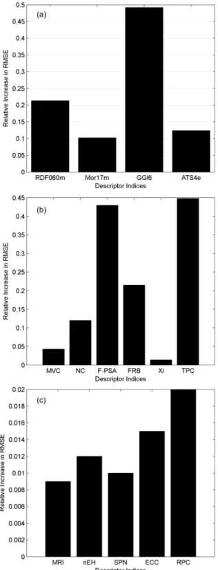
At the end of the BRGNN modeling process a set of the best selected variables were identified, based on their higher frequency in incorporating in the model development. These selected descriptors were then applied to “sensitivity analysis” to measure their relative importance in predictive ability of the model. The results are shown in Table 5. The information contained in this table is more easily seen in the descriptor importance plot shown in Figure 5. The more the RMSE enhancement for each variable demonstrates the more importance of that descriptor in the predictive ability of the model.
The results from sensitivity analysis indicate that Galvez topological charge index of order 634 (GGI6) is
the most important descriptor for describing the rACC1 inhibitory activity, which approximately agrees with the results from the frequency plot in Figure S1a, mentioned earlier. The importance priority of GGI6 in BRGNN model emphasizes its role in modeling the rACC1 activity. Moreover, it is intelligible from the results that although the linear and non-linear models have no descriptors in common, the type of the most important descriptor in both cases is the same, charge indices. Inspection of Figure 5b and 5c shows that the charge descriptors play a major role
Figure 4. The residuals of the calculated pIC50 values against the experimental values for the calibration and prediction sets. (a) rACC1(pIC50); (b) hACC2(pIC50); (c) rACC1 (LE) as dependent variable. MLR’s correlation values, inform that neural networks has performed more accurate than linear models.
for describing the hACC2 inhibitory activities and also rACC1 ligand efficiencies. This outlook may be a guide to find out a trend in the rACC1 inhibitors towards their inhibitory activity which is thereby related to the local charge of compounds.
The appearance of the molecular descriptors of total positive charge (TPC), relative positive charge (RPC), fragment-based polar surface area (F-PSA), unipolarity36
(UniP), polarity number37 (Pol), and GGI6 in the linear and
non-linear QSAR models in this work shows the critical
Table 3. The relative mean effects of the SPA-MLR selected molecular descriptors
Dependent variable Relative mean effect of descriptorsa
rACC1 (pIC50) SubPb 24% MSE 78% UniP 55% CENT 28% More12e 45%
hACC2 (pIC50) RPC 74% MSE 53% DDI 16% X1Sol 23% C-044 35%
rACC1 (LE) TPC 62% Pol 27% Nc 12% X1Sol 19 % GuD 7% UniP 44%
aThe relative mean effects were calculated on a scale between 0 ca 100%. The results are mean values for 100 times repetition of algorithms with random
sets of calibration and prediction sets; bplease see Table S2 in SI section in order to find the meaning of the molecular descriptors.
Table 4. The summary of the SPA-MLR models for modelling the rACC1, hACC2 inhibitory activities
Dependent
variable Intercept Coefficient of the dependent variables
a
rACC1 (pIC50) 3.62 +2.74 SubPb +0.83 MSE –0.21 UniP –1.44 CENT +0.49 More12e
hACC2 (pIC50) 2.75 +3.57 RPC +1.24 MSE –0.73 DDI –0.47 X1Sol +0.63 C-044
rACC1 (LE) 0.27 +1.20 TPC –0.11 Pol +0.28 Nc –0.16 X1Sol +0.15 GuD +0.15 UniP
aThe intercept and coefficients have been calculated after normalizing the molecular descriptors between 1 and –1 values; bplease see Table S2 in SI section
in order to find the meaning of the molecular descriptors.
Table 5. The results of sensitivity analysis on BRGNN’s selected molecular descriptors
Dependent Variable Descriptor RMSE before the scrambling procedure
RMSE after the scrambling procedure
Relative increase in RMSE
rACC1 (pIC50)
RDF060ma 0.336 0.549 0.213
Mor17m 0.336 0.438 0.102
GGI6 0.336 0.828 0.492
ATS4e 0.336 0.460 0.124
hACC2 (pIC50)
MVC 0.407 0.450 0.043
NC 0.407 0.527 0.120
F-PSA 0.407 0.840 0.430
FRB 0.407 0.622 0.215
Xi 0.407 0.421 0.014
TPC 0.407 0.855 0.448
rACC1 (LE)
MRI 0.027 0.036 0.009
nEH 0.027 0.039 0.012
SPN 0.027 0.037 0.010
ECC 0.027 0.042 0.015
RPC 0.027 0.047 0.020
aPlease see Table S2 for the definition of the given molecular descriptors.
role of the charge and polarity of the molecules on their inhibition behavior.
The TPC and RPC descriptors stand for “total” and “relative” positive charge in molecules. The data in Table 3 implies that the contributions of these molecular descriptors on rACC1 (LE) and hACC2 (pIC50) activities
and represents the total amount of charge transfer in the molecules.34 Selection of GGI6 together with TPC and
RPC in this work implies the inhibition mechanism is an electrical based procedure. Regarding the definition of these molecular descriptors, it can be concluded that the positive
charge of molecules has considerable effect on their ACC inhibitory activities and therefore this molecular property should be taken into account for designing novel and potent compounds incorporated in treatment of diabetes type II and metabolite syndrome.
The F-PSA is the fragment-based polar surface area and encodes the surface in molecule belonging to polar atoms. This molecular descriptor was shown to correlate well with passive molecular transport through membranes and, therefore, allows prediction of transport properties of drugs (penetration and intestinal absorption).35 The appearance
of this molecular descriptor in this work highlights the significant role of “diffusion” on ACC inhibitory activity.
The UniP and Pol descriptors are the unipolarity36
and polarity number37 of molecules. These molecular
descriptors can be easily calculated by using the distance matrix of the H-depleted molecular graph.37,38 The polarity
number is the number of pairs of vertices at a topological distance equal to three.37,38 It is usually assumed that the
polarity number accounts for the flexibility of acyclic structures in a molecule. The unipolarity is the minimum value of the vertex distance degrees in a molecular graph. This parameter is inversely related to the local flexibility in molecules.39,40 The data in Table 4, suggests the positive
effect of UniP on ACC inhibitory activity, while it proposes a negative effect for polarity number. These two molecular descriptors emphasize on the role of bond flexibility on the inhibitory activity of studied compounds.
The previous structure-activity relationship studies together with homology modeling and docking investigations have found some similar outlines on ACC inhibitory activities.41-43 These works suggest potent hydrogen bonding
between the carbonyl group adjacent to the anthracene of CP-640186 and the main-chain amide N atom of Glu2230 in ACC structure. Another weak hydrogen bond was observed between the carbonyl group adjacent to the morpholine and the amide N atom of Gly2162 in ACC structure. Singh et al.44
reported a comparative molecular field analysis (CoMFA) and comparative molecular similarity analysis (CoMSIA) for modeling the inhibitory activity of ACC inhibitors. They suggest the critical role of electropositive potential near carbamol functional group on ACC inhibitory activity. Some important spatial steric issues have also been found by them affecting the activity.44 These studies represent the
role of positive charge and shape of molecules on activity of compounds and this is in agreement with our findings.
Conclusions
The main aim of the present work was to develop a QSAR model for predicting the inhibitory activity of the
ACC inhibitors. Since variable selection is a critical step in every QSAR study, four different algorithms based on Monte Carlo cross-validation techniques were investigated. Comparing the results of stepwise-MLR, MLR-ANN, SPA-ANN, GA-MLR, GA-MLR-ANN and BRGNN dedicates that the last model selects the best variables for predicting the inhibition action of ACC inhibitors. In addition to non-linear ANN modeling, the preceding procedure was repeated for linear MLR modeling. A sensitivity analysis was done to characterize the relative importance of descriptors. By representing the most important descriptor in ANN modeling and ranking the present variables by importance, we have reduced the black-box limitation of the neural network methodology, to some extent. The sensitivity analysis of models and relative mean effect of the molecular descriptors in this work have shown that the positive charge of the molecules has considerable effect on their ACC inhibitory activities. This is in agreement with previous studies about the inhibitors of ACC enzyme whish have emphasized on the role of electrostatic interactions on ACC inhibitory activity. Generally, the results of present contribution would help for better understanding the mechanism of the ACC inhibitory activity of arylquinoline amide derivatives and would be useful for medicinal chemists dealing with optimization of this series of compounds.
Supplementary Information
Supplementary data (frequency plot and histograms) are available free of charge at http://jbcs.sbq.org.br as PDF file.
Acknowledgments
I would like to thank Ms. Elham Bakhtiary for her great comments and helpful guidelines in this project.
References
1. Havale, S. H.; Pal, M.; Bio. Med. Chem. 2009, 17, 1783. 2. Wild, S.; Roglic, G.; Green, A.; Diabetes Care 2004, 27, 1047. 3. http://www.who.int/mediacentre/factsheets/fs312/en/, accessed
in February 2015.
4. Kramer, H.; Cao, G.; Dugas, L.; Luke, A.; J. Diabetes Complications2010, 24, 368.
5. Kahn, S. E.; Hull, R. L.; Utzschneider, K. M.; Nature2006,
444, 840.
6. Polakis, S. E.; Guchhait, R. B.; Zwergel, E. E.; Lane, M. D.; Cooper, T. G.; J. Biol. Chem. 1974, 249, 6657.
7. Tong, L.; Harwood, H. J.; J. Cell. Biochem. 2006, 99, 1476. 8. Castle, J. C.; Hara, Y.; Raymond, Ch. K.; Garrett-Engele, Ph.;
Ohwaki, K.; Kan, Zh.; Kusunoki, J.; Johnson, J. M.; Plos One 2009, 4, 4369.
9. Freeman-Cook, K.; Amor, P.; Bader, S.; Buzon, L. M.; Coffey, S. B.; Corbett, J. W.; Dirico, K. J.; Doran, S. D.; Elliott, R. L.; Esler, W.; Guzman-Perez, A.; Henegar, K. E.; Houser, J. A.; Jones, C. A.; Limberakis, C.; Loomis, K.; McPherson, K.; Murdande, S.; Nelson, K. L.; Phillion, D.; Pierce, B. S.; Song, W.; Sugarman, E.; Tapley, S.; Tu, M.; Zhao, Z.; J. Med. Chem. 2012, 55, 935.
10. Corbett, J.; W.; Freeman-Cook, K. D.; Elliott, R.; Vajdos, F.; Rajamohan, F.; Kohls, D.; Marr, E.; Zhang, E.; Tong, L.; Tu, M.; Murdande, S.; Doran, S. D.; Houser, J. A.; Song, W.; Jones, C. J.; Coffey, C. B.; Buzon, L.; Minich, M. L.; Dirico, K. J.; Tapley, S.; McPherson, R. K.; Sugarman, E.; Harwood, H. J.; Esler, W.; Bio. Med. Chem. Lett. 2010, 20, 2383.
11. Jalali-Heravi, M.; Mani-Varnosfaderani, A.; QSAR Comb. Sci.
2009, 28, 946.
12. Winkler, D. A.; Brief Bioinform. 2002, 1, 73.
13. Anderson, C. M.; Bro, R.; J. Chemometr. 2010, 24, 728. 14. Brereton, R. G.; Chemometrics: Data Analysis for the
Laboratory and Chemical Plant; Wiley: New York, 1995. 15. Brown, S. D.; Tauler, R.; Walczale, B.; Comprehensive
Chemometrics; Elsevier, 2009. 16. Leardi, R.; J. Chemometr2001, 15, 559.
17. Fernández, M.; Caballero, J.; Bioorg. Med. Chem. 2007, 15, 6298.
18. Caballero, J.; Tundidor-Camba, A.; Fernández, M.; QSAR Comb. Sci.2007, 26, 27.
19. Caballero, J.; Fernández, M.; González-Nilo, F. D.; Bioorg. Med. Chem. 2008, 16, 6103.
20. Caballero, J.; Garriga, M.; Fernández, M.; Bioorg. Med. Chem.
2006, 14, 3330.
21. Fernández, M.; Caballero, J.; Fernandez, L.; Abreu, J. L.; Garriga, M.; J. Mol. Graphics Modell.2007, 26, 748. 22. Fernández, M.; Abreu, J. L.; Caballero, J.; Garriga, M.;
Fernández, L.; Mol. Simul. 2007, 33, 1045.
23. Fernández, M.; Caballero, J.; Chem. Biol. Drug Des. 2006, 68, 201.
24. Fernández, M.; Carreiras, M. C.; Marco, J. L.; Caballero, J.;
J. Enzyme Inhib. Med. Chem. 2006, 21, 647.
25. Hawkins, D. M.; Kraker, J.; J. Chemometr. 2010, 24, 188. 26. Esbensen, K. H.; Geladi, P.; J. Chemometr. 2010, 24, 168. 27. Guha, R.; Jurs, P. C.; J. Chem. Inform. Model. 2005, 45, 800. 28. Hypercube, Inc.; Hyperchem 7; A professional molecular
modeling environment, USA, 2007.
29. Todeschini R.; Consonni V.; Mauri A.; Pavan M.; Dragon 3 web version: Calculation of Molecular Descriptors, Department of
Environmental Sciences, University of Milan - Bicocca, Italy, 2003.
31. Jalali-Heravi, M.; Mani-Varnosfaderani, A.; SAR QSAR Env. Res. 2011, 22, 293.
32. Roy, P. P.; Paul, S.; Mitra, I.; Roy, K.; Molecules 2009, 14, 1660. 33. Mitra, I.; Saha, A.; Roy, K.; Mol. Simul. 2010, 13, 1067. 34. Deconinck, E.; Zhang, M. H.; Petitet, F.; Dubus, E.; Ijjaali, I.;
Coomans, D.; Anal. Chim. Acta2008, 609, 13.
35. Ertl, P.; Rohde, B.; Selzer, P.; J. Med. Chem. 2000, 43, 3714. 36. Todeschini, R.; Consonni, V.; Handbook of molecular
descriptors, methods and principles in medicinal chemistry, Wiley-VCH: Weinheim, 2000.
37. Platt, R. J.; J. Phys. Chem. 1952, 56, 328. 38. Wiener, H.; J. Phys. Chem. 1947, 69, 17.
39. Lieth, C. W.; Stumpf-Nothof, K.; Prior, U.; J. Chem. Inf. Comput. Sci. 1996, 36, 711.
40. Fechner, N.; Jahn, A.; Hinselmann, G.; Zell, A.; J. Chem. Inf.
Model. 2009, 49, 549.
41. Bhadauriya, A.; Dhoke, G. V.; Gangwal, R. P.; Damre, M. V.; Sangamwar, A. T.; Mol. Diversity2013, 17, 139.
42. Chonan, T.; Tanaka, H.; Yamamoto, D.; Yashiro, M.; Oi, T.; Wakasugi, D.; Ohoka-Sugita, A.; Io, F.; Koretsune, H.; Hiratate, A.; Bioorg. Med. Chem. Lett. 2010, 20, 3965. 43. Yamashita, T.; Kamata, M.; Endo, S.; Yamamoto, M.;
Kakegawa, K.; Watanabe, H.; Miwa, K.; Yamano, T.; Funata, M.; Sakamoto, J. I.; Tani, A.; Mol, C. D.; Zou, H.; Dougan, D. R.; Sang, B.; Snell, G.; Fukatsu, K.; Bioorg. Med. Chem. Lett.
2011, 21, 6314.
44. Singh, U.; Gangwal, R. P.; Dhoke, G. V.; Prajapati, R.; Damre, M.; Sangamwar, A. T.; Arab. J. Chem., in press, DOI: 10.1016/j.arabjc.2012.10.023.
Submitted: September 19, 2014