Mário F. Mucheroni
Andréa Cardoso
[email protected] Departamento de Engenharia Mecânica Escola de Engenharia de São Carlos Universidade de São Paulo 13560-970 São Carlos, SP, BrazilOutput-Only Structural Identification
of Random Vibrating Systems
A new form to carry out stochastic identification of structures in operational conditions using a non recursive method, the statistic analysis and the wavelet transform, is presented. The statistic analysis contributed to select the best system order and to automation of computational procedures. In general the identification of low frequencies is a difficult task. The wavelet transform is an essential tool for compression of data making possible the complete identification including low frequencies. In addition it improves the computational efficiency. The study of four degrees of freedom simulated system is presented and the results are compared with the analytical modal parameters.
Keywords: Operational modal analysis, identification methods, eigensystem realization
algorithm, output-only identification
Introduction
One of the main objectives of Experimental Modal Analysis is Systems Identification. Systems Identification is a name for several methods that build a mathematical model for dynamic systems using input and output data. Nowadays the development of these methods in the time-domain has been applied mainly in the identification of systems with high modal density, especially subspace-based system identification methods applied to the realization systems. They supply reliable state-space models for multivariate systems (Viberg, 1995).1
A modal test with multiple inputs is frequently recommended because it presents more realistic results, although the high cost for its accomplishment. Frequently the structure is tested in laboratory with only one excitation point, that is to say, under boundary conditions different from the real operational conditions. This procedure generally compromises the identification results. The solution of this problem is the accomplishment of the test with the structure in work. In these cases the system is multi-excited and the forces are not totally known. In general, under certain operational conditions, the input data can be approximate to white noise (Desforges, Cooper and Wright, 1995). Therefore the development of methods for study the dynamic behavior of systems excited by random forces becomes important.
James et al (1995) contributed to introduce in mechanical engineering community the idea that it is possible to extract the modal parameters of systems excited by unknown forces. The authors demonstrate that the correlation functions have the same form as impulse response functions and so they can be used in the identification algorithms of traditional Modal Analysis. Classical techniques like Least Squares Complex Exponential (LSCE), Ibrahim Time Domain (ITD), Polyreference Technique (PRCE) and Eigensystem Realization Algorithm (ERA) (Maia et al, 1997) are appropriate to extract the modal parameters from the measured response data of structures undergoing ambient excitation.
In analysis of large flexible structures the ERA presents some advantages. The algorithm finds the model of smallest order that fits the data, within a precision; besides it is an effective method for analysis of structures with close frequencies, with or without noise in the data.
Based on theoretical results of realization theory, Ho and Kalman (1966) developed an algorithm that fits a state-space model of minimum order starting from the dynamic impulse response and based on the concepts of controllability and observability. Later,
Paper accepted September, 2005. Technical Editor: Atila P. Silva Freire.
Juang and Pappa (1985) proposed the incorporation of the singular value decomposition (Golub and Loan, 1989) into Ho-Kalman algorithm, creating the Eigensystem Realization Algorithm, that is a method of balanced realization based on orthogonal subspace decomposition.
This algorithm uses the system response in a special form, called Markov Parameters. Frequently these parameters are obtained from input-output data. The identified model is a representation of the realistic system and can be used to evaluate the natural frequencies and damping factors, as to predict the response of the system when it is excited by different forces.
In this work the algorithm ERA was applied to a simulated system of four degrees of freedom excited by uncorrelated random forces, with non proportional damping matrix, in order to obtain the space-state model of tested structure.
State-Space Representation
Vibration tests are, frequently, performed in order to estimate the modal parameters of a structure that are used in the analysis of its dynamic behavior.
The behavior of many dynamical systems can be expressed by ordinary differential equations. A typical mechanical linear and time-invariant system, with n degrees of freedom, can be characterized by the following second order vectorial differential equation, denominated equation of motion:
( ) ( ) ( ) ( )
Mw t +Zw t +Kw t = f t (1) where t represents the continuous time, M Z K, , ∈Rn n× are the mass, damping and stiffness matrices respectively, f t( )∈Rn×1 is the vector of force or excitation, and 1
( ) n
w t ∈R× is the displacement vector. Note that forcing vector can be written asf t( )=Uu t( ), where
n r
U∈R× describes the r inputs in space and 1
( ) r
u t ∈R× describes them
in time.
The system described by Eq. (1) is equivalent to the following continuous time space-state model:
+ =
+ =
) ( ˆ ) ( ˆ ) (
) ( ˆ ) ( ˆ ) (
t u D t x C t y
t u B t x A t x
(2)
n n Z M K M I A 2 2 1 1 0 ˆ × − − − −
= is the state matrix;
r n U M B × − = 2 1 0
ˆ is the input matrix;
[
LM K LM Z]
m nCˆ 1 1 2
× −
− −
−
= is the output matrix;
[
LM U]
mr Dˆ = −1 ×is the direct transmission matrix;
1 2 ) ( ) ( ) ( × = n t w t w t
x is the state vector;
and L is a matrix which contains information about the location of measurement points relative to the variables in the generalized coordinates. When the output are only measurements in function of the acceleration, L is such that y (t) = L w(t).
In special cases the state variables can be considered as output system. However, usually it is impossible to observe all the state variables directly, for reasons of inaccessibility. In these cases only a set of m output variablesy∈Rm×1, dependent of x (t) and u (t),
can be measured where always m≤n. In this work y t( )is the measurement of the system accelerations in specific structure points at the instant of time t.
For practical purposes, we are concentrated in the situation where the variables are measured only in discrete intervals instead of continuous time, producing the so called Discrete Systems. Therefore the variables are defined at fixed-time intervals:
0, , 2 , , , ( 1) ,
t= ∆ ∆t t k t k∆ + ∆t , where ∆t is constat.
Thus, it is obtained an approximation of the continuous time representation, denominated discrete time state-space model:
+ = + = + k k k k k k u D x C y u B x A x 1 (3) where ) (k t x xk = ∆ ,
t A e
A= ˆ∆ , B=
(
A−I)
Aˆ−1Bˆ , C=Cˆ, D=DˆSolving Eq. (3) for yk, we can write the direct relationship between input and output
∑ + + = = − − k
i ki
i k k
k CA x Du CA Bu y
1 1
0 (4)
Let P0=D and P CA B 1 i i
−
= . Then, we have
∑ + =
= −
k
i i k i k
k CA x Pu y
0
0 (5)
Consider the case where the state matrix A is asymptotically stable. There is a sufficiently large integer p such thatAk≈0, for all
k≥p. Consider the output equation after p time instants:
p k p k p
k Cx Du
y+ = + + + (6)
As it has been done for the original Eq. (3), the following input-output relationship can be obtained:
∑ + = + + + + = = +− + − + − + p
i i k pi k p p k p k k p k p p k u P x A C u D u B C u B A C x A C y 0 1 1 (7)
Since Ak≈0when
k≥pand the observed state vector
[
0 1 − −1]
= x x xl p
X (8)
is limited, the residual effect p k
CA x can be ignored.
If a sufficient number of points from the initial part of the output data set are ignored, Eq. (4) can be written in the following condensed form:
∑
= − = k i i k i k Pu y0
(9)
Therefore the output in any time can be written as a sum of present and past inputs by a weighted sequence of
matrices m r
k
P∈R × , known as Markov parameters. The number p
determines the maximum number of independent Markov parameters. It is important to observe that for each system there is a unique system of Markov parameters. In fact, they are the impulse response, as it is shown, for instance, in Tsunaki (1999). So these parameters represent a complete characterization of the system and can be used as a base for identification of the mathematical model of linear dynamic systems.
Stochastic Identification
The stochastic identification problem deals with the determination of the state-space model using only output data. Starting from identified matrices A and C the modal parameters can be calculated.
It is possible to consider the stochastical components present in data and then the following combined deterministic-stochastic state-space model can be obtained:
+ + = + + = + k k k k k k k k v u D x C y s u B x A x 1 (10)
where the vectors n1 k
s ∈R× and m1 k
v ∈R × are both considered zero
mean white noise. The covariance matrices are given by:
(
)
[ ] [ ]
[ ] [ ]
= ε ε ε ε = ε T S S Q v v s v v s s s v s v s T T q p T q p T q p T q p T q T q p p ´ (11)where
ε
(.)
is the expectation operator.The stochastical systems identification is defined when uk ≡0. Then in cases where the system input can not be measured, it is assumed that the excitation effect is modeled by the disturbances
k
s
andv
k. Then + = + = + k k k k k k v x C y s x A x 1 (12)
The stochastic process
x
k is considered stationary and zeromean, and the noises
s
k andv
kare considered independents of thecurrent state.
Let the output and state-output covariance matrices, respectively, given by
[
T]
k i k i y y
[
T]
k k y x
G=ε +1 (14)
The matrices i
R satisfy the following properties:
1) R C CT T
0= Σ + where
[ ]
T k kx x ε =
Σ is a constant matrix.
In fact,
[
]
[
(
)(
)
]
[ ]
[ ] [ ]
[ ]
T C C v x C x v v x C C x x C v x C v x C y y R T T k k T T k k T k k T T k k T k k k k T k k + Σ = ε + ε + ε + ε = + + ε = ε = 02) R CAi G
i 1
−
= , for i∈ZZZZ and i≥1. In fact,
[
]
[
(
)
]
(
)
[
]
[
]
[
]
[
] [ ]
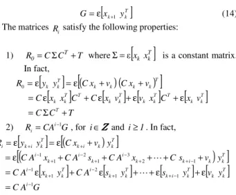
G A C y v y s y s A C y x A C y v s C x A C s A C x A C y v x C y y R i T k k T k i k T k k i T k k i T k k i k k i k i k i T k k i k T k i k i 1 1 1 2 1 1 1 2 3 1 2 1 1 − − + + − + − − + + − + − + − + + = ε + ε + + ε + ε = + + + + + ε = + ε = ε =These properties provide a characterization of the output covariance matrices in function of the matrices A, G, C and R0.
As well as in deterministic models, Markov parameters are used as a base for system identification using ERA algorithm. In the stochastic model the matrices Rican be seen as impulse response and used for system identification instead the originals Markov parameters.
As in the traditional algorithm, Markov parameters was conveniently grouped in two special Hankel matrices, denoted by
0
H
and1
H . We will compose such matrices with the output covariance matrices
i
R. For any natural numbers p and q, we have:
qm pm q p p p q q R R R R R R R R R H × − + + + = 1 1 1 3 2 2 1 0 qm pm q p p p q q R R R R R R R R R H × + + + + + = 2 1 2 4 3 1 3 2 1
Starting from Hankel matrices it is possible to obtain the
matrices
[
]
0
, , ,
A G C R of the stochastic model by applying the ERA algorithm.
Correlation Functions
The correlation function or the corresponding Fourier transform, known as spectral density function, measures the linear dependence degree between two or more data sets. These two functions give the same information, although historically the spectral density function was developed as a tool to solve problems of engineering while the correlation function was mainly used in statistical applications. The first is very popular in the experimental data analysis, however in some applications the second function is shown more convenient.
According to the definition given by Eq.(13) and starting from output data yk in discrete time k=0,1, ,l, the ergodic hypothesis enables the calculation of moment functions of an stationary random process from an unique measurement, sufficiently long to contain all the statistical information of the phenomenon. We have, by definition,
[
]
∑
− = + ∞ → + = ε = 1 0 1 1 lim l k T k k l T k i ki y y
l y
y
R (15)
In practice, the so defined correlation functions are unknown, because only a finite number of data can be measured. Clearly it is necessary to use estimate values. Actually, no random process is truly stationary. However long observations of the process exhibit characteristics that allow them to be considered as stationary. Most of the results obtained in identification of mechanical systems are based
on the steady-state response, which is considered a stationary process satisfying the ergodic hypothesis. The stationary concept of a random process is similar to steady-state behavior of a deterministic process. The unbiased estimate of the correlation function used in this work is given by
∑
−− = + − = 1 0 1ˆ li
k T k i k
i y y
i l
R (16)
We obtain the Hankel matrices Hˆ0 and Hˆ1 changing each
correlation Ri in H0 and H1by the respective estimate ˆRi.
Simulated Model
The simulated data were generated to represent a system of four degrees of freedom, illustrated in Fig.1. The chosen model has non proportional damping matrix in order to generalize the analysis of the identification of systems with linear viscous damping.
Table 1 presents the physical parameters and modal characteristics of the simulated system, where Mi is the modulus of the eigenvalue λi and ϕi is its phase angle.
Figure 1. Four degrees of freedom model.
Table 1. Physical and theoretical modal parameters.
i mi
(kg) zi (N.s/m)
ki
(N/m) λi(rad/s) Mi cosϕi
1 1 8 1000 -0.5472+15.39i 15.40 0.0355
2 5 4 8000 -3.520+95.25i 95.31 0.0369
3 0.5 4 8000 -5.079+104.3i 104.4 0.0486
4 0.25 2 2000 -8.053+154.5i 154.7 0.0520
5 0.2 1000
Non correlated random forces were applied in each one of the masses. The computational precision and the imperfections in the measurement instruments are possible sources of noise. In order to simulate a more realistic situation, an additional white noise was generated and added to the response data. Two levels of noise were considered: 1% and 5%.
The stochastic identification requires a great number of time instants observed. So it is necessary at least 60 seconds of outputs data, recorded in intervals of 0.001 seconds.
One of the most difficult tasks in modal analysis is the determination of the model order. According to Juang and Phan (1994), a trial and error process is required to find the best order. In general, the model order is considerably larger than the real system order, particularly when the data is very noisy. In this case it is said that the model is overdetermined.
Using a overdetermined model, the identification procedure results is a set of structural and computational modes, the first one due to the dynamical characteristics of the structure and the last one due mainly to data-noise and the numeric ill-conditioning.
To apply ERA algorithm is necessary the definition of Hankel matrices
0
H and H1 dimension, given by pm qm× where m is the
number of observed outputs, p and q are arbitrary numbers related to estimated model order. Let be p the system number of independent Markov parameters. It is possible to link the parameters q and p in the following way:
2 p
q= (17)
In this way, p is a unique free parameter in identification procedure. Each value of p determines one data identification that will be named sample. The identification algorithm will be applied consecutively for positive values p increased by 2, taken from an initial value p(i) until a determined limit p(f). The Fig. 2 summarizes
the computational procedures for the storage of samples, where the block named ‘sample’ stores the samples collected for all value of p.
Figure 2. Recursive procedure for storage of the samples identification.
Because the noise is not correlated with the input and output data, it is assure that computational modes tends to change strongly from one to other estimate, while the natural frequencies tend to stabilize in certain intervals within frequency band.
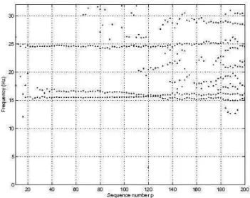
In this study, we obtained 95 identifications varying the number of independent Markov parameters p from 10 to 200. The results of these identifications are schematically represented in Fig.3, where
the plot points correspond to the identified eigenvalues modulus for each p.
Figure 3. Stability of natural frequencies values.
The analysis of the stability diagram presented in Fig. 3 shows that the frequency interval [20,25] has one stable frequency for all variation band of p, while the frequency interval [15,20] presents two stable frequencies for the variation band 10-120 of the parameter p. However it is required a formulation of an analytic criterion for these graphical conclusions.
The statistic moments are fundamental in extraction process of the modal parameters from stationary random signals. Therefore the standard-deviation of the samples in a determined frequency interval characterizes analytically the stability of the identified frequency values. So, high standard-deviation indicates great variability in estimated frequency values while a lithe value of this index reflects the nearly linear behavior in some variation interval of p. These stabilized values characterize the system natural frequencies.
Thus, the statistical analysis applied to a sufficient number of samples can determine the appropriate model order. This rule, applied to simulated data, shows that the estimated model order is 6, what does not correspond to the theoretical model order 8 - the simulated model has 4 degree-of-freedom.
This incorrect order determination happened because the lowest frequency was not identified due to noisy data. To attenuate the effect of the noise in the identification process, as well to perform a different stochastic identification for low frequencies, we choose to analyze the process by frequency bands. So, it was necessary to use low-pass filters to carry out this task without loss of time domain information data.
The Wavelet Transform
The traditional Fourier Transform (FT) does not allow a local analysis of the frequency content in the signal. On the other hand, the Short Time Fourier Transform (STFT) allows an analysis of the frequency of the signal locally in time. However, STFT is not appropriate to analyze certain signals, because the size of the observation window stays constant for all the frequencies.
for high frequencies, the wavelets were moved on small steps, while for low frequencies, the displacement is made with large steps (Vetterli and Kovacevic, 1995).
The mother-wavelet db5 was used is this work for decomposition at level 3 and 2 for bands of low and medium frequencies, respectively. Figure 4 illustrates the decomposition process for the signal of mass 1 acceleration. The reconstruction of
the signal is given by
3 3 2 1
s= + +a d d +d , where
a
3 is the approximation at level 3 andd
i are the details obtained by thesuccessive decompositions.
Figure 4. Decomposition using WT with db5 at level 3.
Because the great number of necessary time instants to carry out the stochastic identification, the WT was fundamental for complete system identification. The WT permits the compression of the information contained in a long data sequence to a short sequences according with the frequency band analyzed.
Numerical Results
The natural frequencies values stabilization give information on
p value optimized for identification process within different frequency bands and noise levels. The wavelet-mother db5 was applied to simulated data in several levels according with the frequency band. The frequency band was divided into three sets called first, second and third order modes. Like this, it was applied db5 level 3 and 2 for low and intermediate frequencies, respectively, and no wavelet transform was applied for high frequency.
Figure 5 summarizes the algorithm developed and illustrates the steps of the method for stochastic identification of structures.
In this way, the identification results are presented in Fig. 6 to 8, with p varying from 10 to 60 for data with 1% of noise at different WT levels.
Figure 5. Flow chart of stochastic identification method.
Figure 6. Stability of low frequencies values with db5 at level 3.
The application of the WT db5 level 3 became possible the identification of a natural frequency in the interval [0,5] Hz, as can be seen in Fig. 6. The other three system natural frequencies cannot be identified using this wavelet level.
Figure 8. Stability of high frequencies values without WT.
In Fig. 7 it is possible to observe the first three frequencies values stabilized, emphasizing the clear separation of the two closed natural frequencies. Despite of the identification of the lowest frequency done with the identification process using WT db5 level 2, the process carried out using level 3 presents better values for the first modal damping factor. It is clearly observed in Fig. 8 that the higher frequencies values stabilize for all p values.
By this method, all system natural frequencies may be identified with high precision. Table 2 presents the identification results for data corrupted by 1% and 5% of noise, where Mi is the eigenvalue modulus in rad/s, and ϕi is the phase angle. The noise level was defined by the quotient (RMS noise)/(RMS response), where RMS is the signal root mean square. In this quotient, RMS of the response is the largest RMS among the four response signals.
Table 2. Identified modal parameters.
Identification with 1% of noise Difference (%) i pi Mi cos ϕi Mi cos ϕi
1 50 15.19 0.0361 1.34 1.59
2 24 95.23 0.0342 0.08 7.43
3 30 104.1 0.0522 0.27 7.32
4 38 154.4 0.0523 0.19 0.50
Identification with 5% of noise Difference (%) i pi Mi cos ϕi Mi cos ϕi
1 44 15.20 0.0371 1.32 4.42
2 28 95.13 0.0339 0.18 8.15
3 30 104.1 0.0529 0.23 8.70
4 36 154.3 0.0518 0.27 0.53
Conclusions
The modal parameters were identified from a Hankel matrix, composed by estimates of the auto-correlation and cross-correlation functions only with the system response data, associated to ERA algorithm and to application of Wavelet Transform.
The use of the correlation functions makes possible the identification without the knowledge of the inputs. The modal parameters were identified, group by group, to obtain the complete identification. The application of the Wavelet Transform was extremely important for the identification of all structural modal parameters in the analyzed frequency band.
The difficulties in model order estimates were solved with a help of statistic analysis. The modal parameters were qualified without the need of modal confidence parameters.
The effectiveness of the new algorithm implementation was checked by the success in the model order selection and in the computation of the modal parameters of a simulated system. It is important to note that there are low and closed eigenvalues in the numerical model presented. Furthermore, it can be concluded that this technique is a good choice for analysis when a great number of experimental data is necessary.
New researches should be accomplished for studying the vibration modes identification and the application of this method in real structures when the excitation is unknown. Efforts should be done in future to study also the nonlinear effects in identification systems.
Acknowledgments
Financial support from the Coordenação de Aperfeiçoamento de Pessoal de Nível Superior (CAPES) is gratefully acknowledged.
References
Desforges, M.J., Cooper, J.E. and Wright, J.R., 1995, “Spectral and modal parameter estimation from output-only measurements”, Mechanical Systems and Signal Processing, Vol. 9, Nr. 2, pp.169-186.
Golub, G.H. and Loan, C.F., 1989, “Matrix computations”, 2.ed, Baltimore: Johns Hopkins University Press, 642 p.
Goupillaud, P., Grossman, A. and Morlet, J., 1985, “Cycle-octave and related transforms in seismic signal analysis”, Geoexploration, Nr. 23, pp.85-102.
Ho, B. and Kalman, R., 1966, “Efficient construction of linear state variable models from input/output functions”, Regelungstechnik, Vol. 14, pp.545-548.
James III, G.H., Carne, T.G. and Lauffer, J.P., 1995, “The natural excitation technique (NExT) for modal parameter extraction from operating structures”, Modal Analysis: the international journal of analytical and experimental modal analysis, Vol. 10, Nr. 4, Oct, pp.260-277.
Juang, J-N. and Pappa, R.S., 1985, “An Eigensystem realization algorithm for modal parameter identification and model reduction”, Journal of Guindance, Vol. 8, Nr. 5, Sept-Oct, pp.620-627.
Juang, J-N. and Phan, M., 1994, “Linear system identification via backward-time observer models”, Journal of Guindance, Control, and Dynamics, Vol. 17, Nr. 3, May-June, pp.505-512.
Maia, N.M.M. et al, 1997, “Experimental Modal Analysis”, Chichester: John Wiley & Sons, 468 p.
Tsunaki, R.H., 1999, “Identificação automatizada de modelos dinâmicos no espaço de estado”, Tese de Doutorado - Escola de Engenharia de São Carlos, Universidade de São Paulo, São Carlos, 143 p.
Vetterli, M. and Kovacevic, J., 1995, “Wavelets and subband coding”, New Jersey: Prentice Hall, 488 p.