Marcelo J. Colaço
Senior Member, ABCM[email protected] Dept. of Mechanical Engineering Military Institute of Engineering – IME Pç. Gen. Tiburcio, 80 22290-270 Rio de Janeiro, RJ, Brazil
Helcio R. B. Orlande
Senior Member, ABCM[email protected] Dept. of Mechanical Engineering – POLI/COPPE Federal University of Rio de Janeiro – UFRJ Cx.Postal 68503 21941-972 Rio de Janeiro, RJ, Brazil
George S. Dulikravich
[email protected] Dept. of Mechanical and Materials Engineering Florida International University College of Engineering, Room EC 3474 10555 West Flagler St., Miami, FL 33174, U.S.A.
Inverse and Optimization Problems in
Heat Transfer
This paper presents basic concepts of inverse and optimization problems. Deterministic and stochastic minimization techniques in finite and infinite dimensional spaces are revised; advantages and disadvantages of each of them are discussed and a hybrid technique is introduced. Applications of the techniques discussed for inverse and optimization problems in heat transfer are presented.
Keywords: Inverse problems, optimization, heat transfer
Introduction
Inverse problems of heat transfer rely on temperature and/or heat flux measurements for the estimation of unknown quantities appearing in the mathematical formulation of physical problems in this field (Tikhonov and Arsenin, 1977; Bech and Arnold, 1977; Alifanov, 1994; Beck et al, 1985; Alifanov et al, 1995; Dulikravich and Martin, 1996; Ozisik and Orlande, 2000; Kurpisz and Nowak, 1995; Woodbury, 2002; Murio, 1993; Trujillo and Busby, 1997). As an example, inverse problems dealing with heat conduction have been generally associated with the estimation of an unknown boundary heat flux, by using temperature measurements taken below the boundary surface. Therefore, while in the classical direct heat conduction problem the cause (boundary heat flux) is given and the effect (temperature field in the body) is determined, the inverse problem involves the estimation of the cause by utilizing the knowledge of the effect. 1
The use of inverse analysis techniques represents a new research
paradigm. The results obtained from numerical simulations and
from experiments are not simply compared a posteriori, but a close synergism exists between experimental and theoretical researchers during the course of study, in order to obtain the maximum information regarding the physical problem under consideration (Beck, 1999). In the recent past inverse problems have evolved from a specific theoretical research topic to an important practical tool of engineering analysis (Tikhonov and Arsenin, 1977; Bech and Arnold, 1977; Alifanov, 1994; Beck et al, 1985; Alifanov et al, 1995; Dulikravich and Martin, 1996; Ozisik and Orlande, 2000; Kurpisz and Nowak, 1995; Woodbury, 2002; Murio, 1993; Trujillo and Busby, 1997; Beck, 1999; Sabatier, 1978; Hensel, 1991;
least three international journals are specifically oriented to the community involved with the solution and application of inverse problems, both from the mathematical and from the engineering points of view. These include: Inverse Problems, Inverse and
Ill-posed Problems and Inverse Problems in Science and Engineering.
The International Conference on Inverse Problems in Engineering:
Theory and Practice is held every three years since 1993. Also,
several other seminars and symposia have been held in different countries in the past, including the International Symposium on
Inverse Problems in Engineering Mechanics in Japan, and the Inverse Problems, Design and Optimization Symposium in Brazil.
More specifically for the heat transfer community, all major conferences in the field such as the International Heat Transfer
Conference have special sessions or mini-symposia dedicated to
inverse problems.
Inverse problems can be solved either as a parameter estimation approach or as a function estimation approach. If some information is available on the functional form of the unknown quantity, the inverse problem can be reduced to the estimation of a few unknown parameters. On the other hand, if no prior information is available on the functional form of the unknown, the inverse problem needs to be regarded as a function estimation approach in an infinite dimensional space of functions (Tikhonov and Arsenin, 1977; Bech and Arnold, 1977; Alifanov, 1994; Beck et al, 1985; Alifanov et al, 1995; Dulikravich and Martin, 1996; Ozisik and Orlande, 2000; Kurpisz and Nowak, 1995; Woodbury, 2002; Murio, 1993; Trujillo and Busby, 1997; Beck, 1999; Sabatier, 1978; Hensel, 1991; Desinov, 1999; Yagola et al, 1999; Ramm et al, 2000; Morozov, 1984; Zubelli, 1999; Kirsch, 1996; Isakov, 1998).
input data, thus requiring special techniques for its solution in order to satisfy the stability condition.
Successful solution of an inverse problem generally involves its reformulation as an approximate well-posed problem and makes use of some kind of regularization (stabilization) technique. Although the solution techniques for inverse problems do not necessarily make use of optimization techniques, many popular methods are nowadays based on them (Tikhonov and Arsenin, 1977; Bech and Arnold, 1977; Alifanov, 1994; Beck et al, 1985; Alifanov et al, 1995; Dulikravich and Martin, 1996; Ozisik and Orlande, 2000; Kurpisz and Nowak, 1995; Woodbury, 2002; Murio, 1993; Trujillo and Busby, 1997; Beck, 1999; Sabatier, 1978; Hensel, 1991; Desinov, 1999; Yagola et al, 1999; Ramm et al, 2000; Morozov, 1984; Zubelli, 1999; Kirsch, 1996; Isakov, 1998).
Despite their similarities, inverse and optimization problems are conceptually different. Inverse problems are concerned with the
identification of unknown quantities appearing in the mathematical formulation of physical problems, by using measurements of the system response. On the other hand, optimization problems generally deal with the minimization or maximization of a certain objective or cost function, in order to find design variables that will result in desired state variables. In addition, inverse and
optimization problems involve other different concepts. For example, the solution technique for an inverse problem is required to cope with instabilities resulting from the noisy measured input data, while for an optimization problem the input data is given by the desired response(s) of the system. In contrast to inverse problems, the solution uniqueness may not be an important issue for optimization problems, as long as the solution obtained is physically feasible and can be practically implemented. Engineering applications of optimization techniques are very often concerned with the minimization or maximization of different quantities, such as minimum weight (e.g., lighter airplanes), minimum fuel consumption (e.g., more economic cars), maximum autonomy (e.g., longer range airplanes), etc. The necessity of finding the maximum or minimum values of some parameters (or functions) can be governed by economic factors, as in the case of fuel consumption, or design characteristics, as in the case of maximum autonomy of an airplane. Sometimes, however, the decision is more subjective, as in the case of choosing a car model. In general, different designs can be idealized for a given application, but only a few of them will be economically viable. The best design is usually obtained by some Min-Max technique.
In this paper we address solution methodologies for inverse and single-objective optimization problems, based on minimization techniques. Several gradient and stochastic techniques are introduced, together with their basic implementation steps and algorithms. We present some deterministic methods, such as the Conjugate Gradient Method, the Newton Method and the Davidon-Fletcher-Powell Method (Tikhonov and Arsenin, 1977; Bech and Arnold, 1977; Alifanov, 1994; Beck et al, 1985; Alifanov et al, 1995; Dulikravich and Martin, 1996; Ozisik and Orlande, 2000; Kurpisz and Nowak, 1995; Woodbury, 2002; Murio, 1993; Trujillo and Busby, 1997; Beck, 1999; Daniel, 1971; Jaluria, 1998; Stoecker, 1989; Belegundu and Chandrupatla, 1999; Fletcher, 2000; Powell, 1977; Fletcher and Reeves, 1964; Hestenes and Stiefel, 1952; Polak, 1971; Beale, 1972; Davidon, 1959; Fletcher and Powell, 1963; Broyden, 1965; Broyden, 1967; Levenberg, 1944; Marquardt, 1963; Bard, 1974; Dennis and Schnabel, 1983; Moré, 1977). In addition, we present some of the most promising stochastic approaches, such as the Simulated Annealing Method (Corana et al, 1987; Goffe et al, 1994), the Differential Evolutionary Method (Storn and Price, 1996), Genetic Algorithms (Goldberg, 1989; Deb, 2002) and the Particle Swarm Method (Kennedy and Eberhart, 1995; Kennedy, 1999; Naka et al, 2001; Eberhart et al, 2001; Dorigo and Stützle,
2004). Deterministic methods are in general computationally faster than stochastic methods, although they can converge to a local minima or maxima, instead of the global one. On the other hand, stochastic algorithms can ideally converge to a global maxima or minima, although they are computationally slower than the deterministic ones. Indeed, the stochastic algorithms can require thousands of evaluations of the objective functions and, in some cases, become non-practical. In order to overcome these difficulties, we will also discuss the so-called hybrid algorithm, which takes advantage of the robustness of the stochastic methods and of the fast convergence of the deterministic methods (Colaço et al, 2003a; Colaço et al, 2004; Colaço et al, 2003b; Dulikravich et al, 2003a; Dulikravich et al, 2003b; Dulikravich et al, 2003c; Dulikravich et al, 2004; Colaço et al, 2003c). Each technique provides a unique approach with varying degrees of convergence, reliability and robustness at different cycles during the iterative minimization procedure. A set of analytically formulated rules and switching criteria can be coded into the program to automatically switch back and forth among the different algorithms as the iterative process advances. Specific concepts for inverse and optimization problems are discussed and several examples in heat transfer are given in the paper.
Objective Function
Basic Concept
For the solution of inverse problems, as considered in this paper, we make use of minimization techniques that are of the same kind of those used in optimization problems. Therefore, the first step in establishing a procedure for the solution of either inverse problems or optimization problems is thus the definition of an objective
function. The objective function is the mathematical representation
of an aspect under evaluation, which must be minimized (or maximized). It can be mathematically stated as
( )
{
x x xN}
U
U= x; x= 1, 2,..., (1)
where x1, x2, … , xN are the variables of the problem under consideration that can be modified in order to find the minimum value of the function U.
The relationship between U and x can, most of the times, be expressed by a physical / mathematical model. However, in some cases this relationship is impractical or even impossible and the variation of U with respect to x must be determined by experiments.
Constraints
Usually the variables x1, x2, … , xN which appear on the objective function formulation are only allowed to vary between some pre-specified ranges. Such constraints are, for example, due to physical or economical limitations.
We can have two types of constraints. The first one is the
equality constraint, which can be represented by
( )
=α=Gx
G (2.a)
This kind of constraint can represent, for example, the pre-specified power of an automobile.
The second type of constraint is called inequality constraint and it is represented by
( )
≤α=Gx
This can represent, for example, the maximum temperature allowed in a gas turbine engine.
Optimization Problems
For optimization problems, the objective function U can be, for example, the fuel consumption of an automobile and the variables
x1, x2, … , xN can be the aerodynamic profile of the car, the material of the engine, the type of wheels used, the distance from the floor, etc.
Inverse Problems and Regularization
For inverse problems, the objective function usually involves the squared difference between measured and estimated variables of the system under consideration. As a result, some statistical aspects regarding the unknown parameters and the measured errors need to be examined in order to select an appropriate objective function. In the examples presented below we assume that temperature measurements are available for the inverse analysis. The eight standard assumptions (Beck and Arnold, 1977) regarding the
statistical description of the problem are:
1. The errors are additive, that is,
i i i T
Y= +ε (3.a)
where Yi is the measured temperature, Ti is the actual temperature and εi is the random error.
2. The temperature errors εi have a zero mean, that is,
0 ) (i =
Eε (3.b)
where E(·) is the expected value operator. The errors are then said to be unbiased.
3. The errors have constant variance, that is,
constant }
)] (
{[ 2 2
2= − =σ =
σi E Yi EYi (3.c)
which means that the variance of Yi is independent of the measurement.
4. The errors associated with different measurements are uncorrelated. Two measurement errors εi and εj , where i ≠ j, are uncorrelated if the covariance of εi and εj is zero, that is,
0 )]} ( )][ ( {[ ) , (
covεiεj ≡E εi−Eεi εj−Eεj = for i ≠ j (3.d) Such is the case if the errors εi and εj have no effect on or relationship to each other.
5. The measurement errors have a normal (Gaussian) distribution. By taking into consideration the assumptions 2, 3 and 4 above, the probability distribution function of εi is given by
−
= 22
2 exp 2 1 ) (
σ ε π σ
ε i
i
f (3.e)
6. The statistical parameters describing εi , such as σ , are known.
7. The only variables that contain random errors are the
8. There is no prior information regarding the quantities to be estimated, which can be either parameters or functions. If such information exists, it can be utilized to obtain improved estimates.
If all of the eight statistical assumptions stated above are valid, the objective function, U, that provides minimum variance estimates is the ordinary least squares norm (Beck and Arnold, 1977) (i.e., the sum of the squared residuals) defined as
)] x ( T Y [ )] x ( T Y [ ) x
( = − T −
U (4)
where Y and T(x) are the vectors containing the measured and estimated temperatures, respectively, and the superscript T indicates the transpose of the vector. The estimated temperatures are obtained from the solution of the direct problem with estimates for the unknown quantities.
If the values of the standard deviations of the measurements are quite different, the ordinary least squares method does not yield minimum variance estimates (Beck and Arnold, 1977). In such a case, the objective function is given by the weighted least squares
norm, Uw, defined as
)] x ( T Y [ W )] x ( T Y [ ) x
( = − T −
W
U (5)
where W is a diagonal weighting matrix. Such matrix is taken as the inverse of the covariance matrix of the measurement errors in cases where the other statistical hypotheses remain valid (Beck and Arnold, 1977).
If we consider that some information regarding the unknown parameters is available, we can use the maximum a posteriori
objective function in the minimization procedure (Beck and Arnold,
1977). Such an objective function is defined as:
[
Y T(x)] [
WY T(x)]
( x) V ( x)) x
( = − T − + µµµµ− T −1µµµµ− MAP
U (6)
where x is assumed to be a random vector with known mean µµµµ and known covariance matrix V. Therefore, the mean µµµµ and the covariance matrix V provide a priori information regarding the parameter vector x to be estimated. Such information can be available from previous experiments with the same experimental apparatus or even from the literature data. By assuming the validity of the other statistical hypotheses described above regarding the experimental errors, the weighting matrix W is given by the inverse of the covariance matrix of the measurement errors (Beck and Arnold, 1977).
If the inverse heat transfer problem involves the estimation of only few unknown parameters, such as the estimation of a thermal conductivity value from the transient temperature measurements in a solid, the minimization of the objective functions given above can be stable. However, if the inverse problem involves the estimation of a large number of parameters, such as the recovery of the unknown transient heat flux components f(ti) ≡ fi at times ti, i=1,…,I, excursion and oscillation of the solution may occur. One approach to reduce such instabilities is to use the procedure called Tikhonov’s
regularization (Tikhonov and Arsenin, 1977; Bech and Arnold,
where α* (> 0) is the regularization parameter and the second
summation on the right is the whole-domain zeroth-order
regularization term. In Eq. (7.a), fi is the heat flux at time ti , which is supposed to be constant in the interval ti−∆t/2 < t < ti + ∆t/2, where ∆t is the time interval between two consecutive
measurements. The values chosen for the regularization parameter α* influence the stability of the solution as the minimization of Eq.
(7.a) is performed. As α*→0 the solution may exhibit oscillatory behavior and become unstable, since the summation of fi2 terms may
attain very large values and the estimated temperatures tend to match those measured. On the other hand, with large values of α*
the solution is damped and deviates from the exact result.
The whole-domain Tikhonov’s first-order regularization procedure involves the minimization of the following modified least squares norm:
∑ ∑
=
−
= +−
+ − =I
i
I
i i i i
i T f f
Y t f U
1
1
1 2 1 2
) ( * ) ( )] (
[ α (7.b)
For α*→0, exact matching between estimated and measured
temperatures is obtained as the minimization of U[f(t)] is performed and the inverse problem solution becomes unstable. For large values of α*, when the second summation in Eq. (7.b) is dominant, the heat
flux components fi tend to become constant for i = 1, 2, ..., I, that is, the first derivative of f(t) tends to zero. Instabilities on the solution can be alleviated by proper selection of the value of α*. Tikhonov
(Tikhonov, 1977) suggested that α* should be selected so that the
minimum value of the objective function would be equal to the sum of the squares of the errors expected for the measurements, which is know as the Discrepancy Principle.
Alternative approaches for Tikhonov’s regularization scheme described above is the use of Beck’s Sequential Function
Specification Method (Beck et al, 1985) or of Alifanov’s Iterative Regularization Methods (Alifanov, 1994; Alifanov et al, 1995;
Ozisk and Orlande, 2000). Beck’s sequential function specification method is a quite stable inverse analysis technique. This is due to the averaging property of the least-squares norm and because the measurement at the time when the heat flux is to be estimated, is used in the minimization procedure together with few measurements taken at future time steps (Beck et al, 1985). In Alifanov’s regularization methods, the number of iterations plays the role of the regularization parameter α* and the stopping criterion is so chosen that reasonably stable solutions be obtained. Therefore, there is no need to modify the original objective function, as opposed to Tikhonov’s or Beck’s approaches. The iterative regularization approach is sufficiently general and can be applied to both parameter and function estimations, as well as to linear and non-linear inverse problems (Alifanov, 1994; Alifanov et al, 1995; Ozisk and Orlande, 2000).
Minimization Techniques
In this section, we present deterministic and stochastic techniques for the minimization of an objective function U(x) and the identification of the parameters x1, x2, … , xN, which appear on the objective function formulation. Basically, this type of minimization problem is solved in a space of finite dimension N, which is the number of unknown parameters. For many minimization problems, the unknowns cannot be recast in the form of a finite number of parameters and the minimization needs to be performed in an infinite dimensional space of functions (Tikhonov and Arsenin, 1977; Bech and Arnold, 1977; Alifanov, 1994; Beck et al, 1985; Alifanov et al, 1995; Dulikravich and Martin, 1996; Ozisik and Orlande, 2000; Kurpisz and Nowak, 1995; Woodbury, 2002; Murio, 1993; Trujillo and Busby, 1997; Beck, 1999; Sabatier, 1978;
Hensel, 1991; Desinov, 1999; Yagola et al, 1999; Ramm et al, 2000; Morozov, 1984; Zubelli, 1999; Kirsch, 1996; Isakov, 1998; Hadamard, 1923; Daniel, 1971). A powerful and straightforward technique for the minimization in a functional space is the conjugate gradient method with adjoint problem formulation (Alifanov, 1994; Alifanov et al, 1995; Ozisk and Orlande, 2000; Daniel, 1971). Therefore, this technique is also described below, as applied to the solution of an inverse problem of function estimation.
Deterministic Methods
These types of methods, as applied to non-linear minimization problems, generally rely on establishing an iterative procedure, which, after a certain number of iterations, will hopefully converge to the minimum of the objective function. The iterative procedure can be written in the following general form (Beck and Arnold, 1977; Alifanov, 1994; Alifanov et al, 1995; Jaluria, 1998; Stoecker, 1989; Belegundu and Chandrupatla, 1999; Fletcher, 2000; Bard, 1974; Dennis and Schnabel, 1983):
k k k k
d x
x+1= +α (8)
where x is the vector of design variables, α is the search step size, d is the direction of descent and k is the number of iterations.
An iteration step is acceptable if Uk+1 < Uk. The direction of descent d will generate an acceptable step if and only if there exists a positive definite matrix R, such that d=−R∇U(Bard, 1974).
In fact, such requirement results in directions of descent that form an angle greater than 90o with the gradient direction. A minimization method in which the directions are obtained in this manner is called an acceptable gradient method (Bard, 1974).
A stationary point of the objective function is one at which 0
U
∇ = . The most that we can hope about any gradient method is that it converges to a stationary point. Convergence to the true minimum can be guaranteed only if it can be shown that the objective function has no other stationary points. In practice, however, one usually reaches the local minimum in the valley where the initial guess for the iterative procedure was located (Bard, 1974).
Steepest Descent Method
In this section we will introduce the most basic gradient method, which is the Steepest Descent Method. The basic idea of this method is to move downwards on the objective function along the direction of highest variation, in order to locate its minimum value. Therefore, the direction of descent is given by
) x (
dk=−∇U k (9)
since the gradient direction is the one that gives the fastest increase of the objective function. Despite being the natural choice for the direction of descent, the use of the gradient direction is not very efficient. Usually the steepest-descent method starts with large variations in the objective function, but, as the minimum value is reached, the convergence rate becomes very low.
interpolation (Jaluria, 1988; Stoecker, 1989; Belegundu and Chandrupatla, 1999; Fletcher, 2000; Bard, 1974; Dennis and Schnabel, 1983).
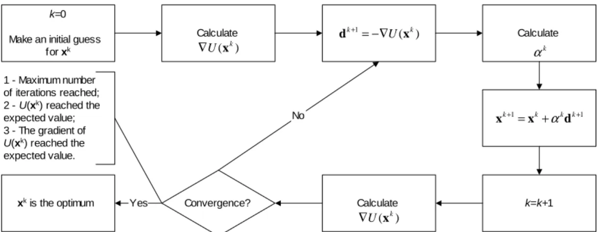
Figure 1 illustrates the iterative procedure for the Steepest Descent Method.
k=0
Make an initial guess for xk
) (
1 k
k
U x
d+ =−∇
Calculate
) ( k
U x
∇
k=k+1
1
1 +
+ = k+ k k
k
d x
x α
Calculate k
α
Calculate
) ( k
U x
∇
Convergence? xk is the optimum Yes
No 1 - Maximum number
of iterations reached; 2 - U(xk) reached the
expected value; 3 - The gradient of
U(xk) reached the
expected value.
Figure 1. Iterative procedure for the Steepest Descent Method.
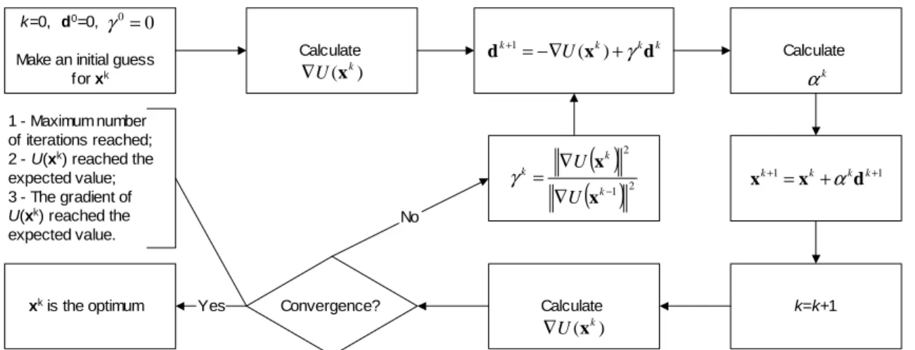
Conjugate Gradient Method
The Conjugate Gradient Method improves the convergence rate of the Steepest Descent Method, by choosing directions of descent that are a linear combination of the gradient direction with directions of descent of previous iterations (Alifanov, 1994; Alifanov et al, 1995; Ozisik and Orlande, 2000; Daniel, 1971; Jaluria, 1998; Stoecker, 1989; Belegundu and Chandrupatla, 1999; Fletcher, 2000; Powell, 1977; Fletcher and Reeves, 1964; Hestenes and Stiefel, 1952; Polak, 1971, Beale, 1972; Davidon, 1959). In a general form, the direction of descent is given by:
( )
k k k k qk
d d x
d =−∇ +γ −1+ψ (10)
where γk and ψk are the conjugation coefficients. This direction of descent is used in the iterative procedure specified by Eq. (8).
The superscript q in Eq. (10) denotes the iteration number where a restarting strategy is applied to the iterative procedure of the conjugate gradient method. Restarting strategies were suggested for the conjugate gradient method of parameter estimation in order to improve its convergence rate (Powell, 1977).
Different versions of the Conjugate Gradient Method can be found in the literature depending on the form used for the computation of the direction of descent given by Eq. (10) (Alifanov, 1994; Alifanov et al, 1995; Ozisik and Orlande, 2000; Daniel, 1971; Jaluria, 1998; Stoecker, 1989; Belegundu and Chandrupatla, 1999; Fletcher, 2000; Powell, 1977; Fletcher and Reeves, 1964; Hestenes and Stiefel, 1952; Polak, 1971, Beale, 1972; Davidon, 1959). In the Fletcher-Reeves version, the conjugation coefficients γk and ψ k are obtained from the following expressions:
( )
( )
1 22
x x
−
∇ ∇ =
k k k
U U
γ , with γ0 = 0 for k=0 (11.a)
( )
[
( ) ( )
]
( )
21
1
x
x x ] x [
−
−
∇
∇ − ∇ ∇ =
k
k k T k k
U
U U U
γ ,
with γ0 = 0 for k=0 (12.a)
0
=
k
ψ , for k = 0,1,2,… (12.b) Based on previous work by Beale (Beale, 1972), Powell (Powell, 1977) suggested the following expressions for the conjugation coefficients, which gives the so-called Powell-Beale’s version of the Conjugate Gradient Method:
)] x ( ) x ( [ ] d [
)] x ( ) x ( [ )] x ( [
1 1
1
− −
−
∇ − ∇
∇ − ∇ ∇
= k kTT kk kk
k
U U
U U U
γ ,
with γ0 = 0 for k=0 (13.a)
)] x ( ) x ( [ ] d [
)] x ( ) x ( [ )] x ( [
1 1
q q
T q
q q
T k k
U U
U U
U
∇ − ∇
∇ − ∇ ∇
= + +
ψ ,
with ψ0 = 0 for k=0 (13.b)
In accordance with Powell (Powell, 1977), the application of the conjugate gradient method with the conjugation coefficients given by Eqs. (13.a,b) requires restarting when gradients at successive iterations tend to be non-orthogonal (which is a measure of the local non-linearity of the problem) and when the direction of descent is not sufficiently downhill. Restarting is performed by making ψk=0 in Eq. (10).
The non-orthogonality of gradients at successive iterations is tested by the following equation:
(
)
( )
21)] (x ) 0.2 x
x (
[ k T k k
ABS ∇ − ∇ ≥ ∇ (14.a)
where ABS (.) denotes the absolute value.
( )
( )
2x 8 . 0 x ] d
[ kT∇ k ≥− ∇ k (14.c)
We note that the coefficients 0.2, 1.2 and 0.8 appearing in Eqs. (14.a-c) are empirical and are the same used by Powell (Powell, 1977).
In Powell-Beale’s version of the conjugate gradient method, the direction of descent given by Eq. (10) is computed in accordance with the following algorithm for k ≥ 1 (Powell, 1977):
STEP 1: Test the inequality (14.a). If it is true set q = k-1. STEP 2: Compute γk with Eq. (13.a).
STEP 3: If k = q+1 set ψk = 0. If k ≠ q+1 compute ψk with Eq. (13.b).
STEP 4: Compute the search direction dk with Eq. (10). STEP 5: If k ≠ q+1 test the inequalities (14.b,c). If either one of them is satisfied set q = k-1 and ψk=0. Then recompute the search direction with Eq. (10).
The Steepest Descent Method, with the direction of descent given by the negative gradient equation, would be recovered with γk
=ψk=0 for any k in Eq. (10). The same procedures used for the evaluation of the search step size in the Steepest Descent Method are employed for the Conjugate Gradient Method.
Figure 2 shows the iterative procedure for the Fletcher-Reeves version of the Conjugate Gradient Method.
k=0, d0=0,
Make an initial guess for xk
k k k k
U x d
d+1=−∇ ( )+γ
Calculate
) ( k
U x ∇
k=k+1
1
1 +
+ = k+ k k
k
d x
x α
Calculate k
α
Calculate
) ( k
U x ∇
Convergence?
xk is the optimum Yes
No 1 - Maximum number
of iterations reached; 2 - U(xk) reached the
expected value; 3 - The gradient of
U(xk) reached the
expected value.
0 0= γ
( )
( )
1 22
− ∇
∇ =
k k k
U U
x x γ
Figure 2. Iterative procedure for the Fletcher-Reeves version of the Conjugate Gradient Method.
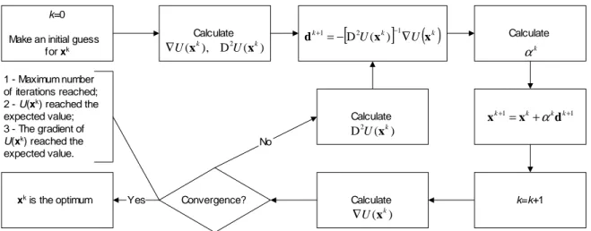
Newton-Raphson Method
While the Steepest Descent and the Conjugate Gradient Methods use gradients of the objective function in their iterative procedures, the Newton-Raphson Method also uses information of the second derivative of the objective function in order to achieve a faster convergence rate (which doesn’t mean a lower computational cost).
Let us consider an objective function U(x), which is, at least, twice differentiable. The Taylor expansion of U(x) around a vector xk, where x – xk = h, is given by (Beck, 1977; Jaluria, 1998; Belegundu and Chandrupatla, 1999; Broyden, 1965; Broyden, 1967; Levenberg, 1944; Marquardt, 1963; Bard, 1974; Dennis and Schnabel, 1983):
( )
2( )
3h h ) x ( D h 2 1 h x ) x ( ) h x
( U U U O
U k+ = k +∇ kT + T k + (15)
where ∇U(x) is the gradient (vector of 1st order derivatives) of the objective function and D2U(x) is the Hessian (matrix of 2nd order derivatives) of the objective function.
If the objective function U(x) is twice differentiable, the Hessian is symmetric, and we can write
( )
x D (x )h )h x
( k U k 2U k
U + ≅∇ +
∇ (16)
A necessary condition for the minimization of the objective function is that its gradient vanishes. Therefore, from Eq. (16) we have:
[
DU(xk)] ( )
Uxkh≅− 2 −1∇ (17)
and the vector that locally optimizes the function U(x) is given by
[
k] ( )
kk DU(x ) Ux x
x≅ − 2 −1∇ (18)
Therefore, the iterative procedure of the Newton-Raphson method, given by Eq. (18), can be written in the same form of Eq. (8) by setting αk=1 and
[
k]
( )
k kU
U(x ) x
D
d =− 2 −1∇ (19)
However, the Newton-Raphson method converges to the extreme point closer to the initial guess, disregarding if it is a maximum, a minimum or a saddle point. For this reason it is common to introduce a search step size to be taken along the direction of descent for this method, so that it is written as:
[
k]
( )
k kk
U
U(x ) x
D
d =−α 2 −1∇ (20)
Figure 3 shows the iterative procedure for the Newton-Raphson Method.
k=0
Make an initial guess for xk
Calculate
) ( D ),
( k 2U k
U x x
∇
k=k+1
1
1 +
+ = k+ k k k
d x
x α
Calculate k
α
Calculate
) ( k
U x ∇
Convergence?
xk is the optimum Yes
No 1 - Maximum number
of iterations reached; 2 - U(xk) reached the
expected value; 3 - The gradient of
U(xk) reached the
expected value.
Calculate
[
k]
( )
kk
U
U x x
d+1=−D2 ( )−1∇
) ( D2 k
U x
Figure 3. Iterative procedure for the Newton-Raphson Method.
Quasi-Newton Methods
In these types of methods, the Hessian matrix appearing in the Newton-Raphson’s Method is approximated in such a way that it does not involve second derivatives. Usually, the approximations for the Hessian are based on first derivatives. As a result, the Quasi-Newton Methods have a slower convergence rate than the Quasi- Newton-Raphson Method, but they are computationally faster (Beck, 1977; Jaluria, 1998; Belegundu and Chandrupatla, 1999; Broyden, 1965; Broyden, 1967; Levenberg, 1944; Marquardt, 1963; Bard, 1974; Dennis and Schnabel, 1983).
Let us define a new matrix H, which is an approximation for the inverse of the Hessian, that is,
[
2]
1) x ( D
Hk≅ U k − (21)
The direction of descent for the Quasi-Newton methods is thus given by:
( )
k k kU x
H
d +1=− ∇ (22)
and the matrix H is iteratively calculated as
1 1
1 M N
H
Hk= k− + k− + k− for k = 1,2,… (23.a)
I
Hk= for k = 0 (23.b)
where I is the identity matrix. Note that, for the first iteration, the method starts as the Steepest Descent Method.
Different Quasi-Newton methods can be found in the literature depending on the choice of the matrices M and N. For the
Davidon-Fletcher-Powell (DFP) Method (Davidon, 1959; Fletcher and Powell, 1963), such matrices are given by
( )
( )
1 11 1 1 1
Y d
d d M
− −
− − − − =
k T k
T k k k
k α (24.a)
(
)(
)
( )
1 1 11 1 1 1 1
Y H Y
Y H Y H N
− − −
− − − − − =−
k k T k
T k k k k
k (24.b)
where
( ) ( )
11
x x
Yk− =∇U k −∇U k− (24.c)
Note that, since the matrix H is iteratively calculated, some errors can be propagated and, in general, the method needs to be restarted after some number of iterations. Also, since the matrix M depends on the choice of the search step size α, the method is very sensitive to its choice. A variation of the DFP method is the Broyden-Fletcher-Goldfarb-Shanno (BFGS) Method (Davidon, 1959; Fletcher and Powell, 1963; Broyden, 1965; Broyden, 1967), which is less sensitive to the choice of the search step size. For this method, the matrices M and N are calculated as
( )
( )
( )
1( )
11 1
1 1
1 1 1 1
Y d
d d
d Y
Y H Y 1 M
− −
− −
− −
− − − −
+
=
k T k
T k k
k T k
k k T k
k (25.a)
( )
( )
( )
1 11 1 1 1 1 1 1
d Y
d Y H H Y d N
− −
− − − − − −
− =− +
k T k
T k k k k T k k
k (25.b)
k=0, H=I
Make an initial guess for xk
Calculate
) ( k
U x
∇
k=k+1
1
1 +
+ = k+ k k
k
d x
x α
Calculate k
α
Calculate
) ( k
U x
∇
Convergence? xk is the optimum Yes
No 1 - Maximum number
of iterations reached; 2 - U(xk) reached the
expected value; 3 - The gradient of
U(xk) reached the
expected value.
( )
k k kUx H d+1=− ∇
( )
( )
11 −
− =∇ k −∇ k
k
U
Ux x
Y
( )
( )
( )
1( )
1 1 11 1
1 1 1
1 1
− −
− −
− −
− − − −
+
=
k T k
T k k
k T k
k k T k k
Y d
d d
d Y
Y H Y M
( )
( )
( )
1 1 1 1 1 1 1 1 1− −
− − − − − −
− =− +
k T k
T k k k k T k k k
d Y
d Y H H Y d
N k= k−1+ k−1+ k−1
N M H H
Figure 4. Iterative procedure for the BFGS Method.
Levenberg-Marquardt Method
The Levenberg-Marquardt Method was first derived by Levenberg (Levenberg, 1944) in 1944, by modifying the ordinary least squares norm. Later, in 1963, Marquardt (Marquardt, 1963) derived basically the same technique by using a different approach. Marquardt’s intention was to obtain a method that would tend to the Gauss method in the neighborhood of the minimum of the ordinary least squares norm, and would tend to the steepest descent method in the neighborhood of the initial guess used for the iterative procedure. This method actually converts a matrix that approximates the Hessian into a positive definite one, so that the direction of descent is acceptable.
The method rests on the observation that if P is a positive definite matrix, then A + λ P is positive definite for sufficiently large λ. If A is an approximation for the Hessian, we can choose P as a diagonal matrix whose elements coincide with the absolute values of the diagonal elements of A (Bard, 1974).
The direction of descent for the Levenberg-Marquardt method is given by (Bard, 1974):
) x ( ) P A (
dk=− k+λk k−1∇U k (26) and the step size is taken as αk = 1. Note that for large values of λk a small step is taken along the negative gradient direction. On the other hand, as λk tends to zero, the Levenberg-Marquardt method tends to an approximation of Newton’s method based on the matrix A. Usually, the matrix A is taken as that for the Gauss method (Beck, 1977; Ozisik and Orlande, 2000; Bard, 1974).
Evolutionary and Stochastic Methods
In this section some Evolutionary and Stochastic Methods like Genetic Algorithms, Differential Evolution, Particle Swarm and Simulated Annealing will be discussed. Evolutionary methods, in opposition to the deterministic methods, don’t rely, in general, on strong mathematical basis and do not make use of the gradient of the objective function as a direction of descent. They tend to mimic nature in order to find the minimum of the objective function, by selecting, in a fashionable and organized way, the points where such function is going to be computed.
Genetic Algorithms
Genetic algorithms are heuristic global optimization methods that are based on the process of natural selection. Starting from a randomly generated population of designs, the optimizer seeks to produce improved designs from one generation to the next. This is accomplished by exchanging genetic information between designs in the current population, in what is referred to as the crossover operation. Hopefully this crossover produces improved designs, which are then used to populate the next generation (Goldberg, 1989; Deb, 2002).
The genes themselves are often encoded as binary strings though they can be represented as real numbers. The length of the binary string determines how precisely the value, also know as the allele of the gene, is represented.
The genetic algorithm applied to an optimization problem proceeds as follows. The process begins with an initial population of random designs. Each gene is generated by randomly generating 0’s and 1’s. The chromosome strings are then formed by combining the genes together. This chromosome defines the design. The objective function is evaluated for each design in the population. Each design is assigned a fitness value, which corresponds to the value of the objective function for that design. In the case of minimization, a higher fitness is assigned to designs with lower values of the object function.
Next, the population members are selected for reproduction, based upon their fitness. The selection operator is applied to each member of the population. The selection operator chooses pairs of individuals from the population who will mate and produce offspring. In the tournament selection scheme, random pairs are selected from the population and the individual with the higher fitness of each pair is allowed to mate.
Once a mating pair is selected, the crossover operator is applied. The crossover operator essentially produces new designs or offspring by combining the genes from the parent designs in a stochastic manner. In the uniform crossover scheme, it is possible to obtain any combination of the two parent’s chromosomes. Each bit in each gene in the chromosome is assigned a probability that crossover will occur (for example, 50 % for all genes). A random number between 0 and 1 is generated for each bit in each gene. If a number greater than 0.5 is generated then that bit is replaced by the corresponding bit in the gene from the other parent. If it is less than 0.5, the original bit in the gene remains unchanged. This process is repeated for the entire chromosome for each of the parents. When complete, two offspring are generated, which may replace the parents in the population.
The mutation process follows next. When the crossover procedure is complete and a new population is formed, the mutation operator is applied. Each bit in each gene in the design is subjected to a chance for a change from 0 to 1, or vice versa. The chance is known as the mutation probability, which is usually small. This introduces additional randomness into the process, which helps to avoid local minima. Completion of the mutation process signals the end of a design cycle. Many cycles may be needed before the method converges to an optimum design.
For more details or for the numerical implementation of Genetic Algorithms, the reader is referred to (Goldberg, 1989; Deb, 2002).
Differential Evolution
The Differential Evolution Method is an evolutionary method based on Darwin’s Theory for the Evolution of the Species. It was created in 1995 by two researchers from Berkeley (Kenneth Price and Rainer Storn) (Storn and Price, 1996) as an alternative to the Genetic Algorithm Method. Following the Theory for the Evolution of the Species, the strongest members of a population will be more capable to survive in a certain environmental condition. During the matting process, the chromosomes of two individuals of the population are combined in a process called crossover. During this process mutations can occur, which can be good (individual with a better objective function) or bad (individual with a worst objective function). The mutations are used as a way to escape from local minima. However, their excessive usage can lead to a non-convergence of the method.
The method starts with a randomly generated population in the domain of interest. Then, successive combinations of chromosomes and mutations are performed, creating new generations until an optimum value is found.
The iterative process of the Differential Evolution Method is given by:
(
)
[
α β γ]
x
x 1 2
1= + + −
+ k F
i k
i δ δ (27)
where
xi is the i-th individual vector of parameters.
α αα
α, ββββ and γγγγ are three members of the population matrix P, randomly chosen.
F is a weight function, which defines the mutation (0.5 < F < 1). k is the number of generations.
δ1 and δ2 are Dirac delta functions that define the mutation.
In the minimization process, if U(xk+1) < U(xk), then xk+1 replaces xk in the population matrix P. Otherwise, xk is kept in the population matrix.
The binomial crossover is given as
> < =
CR R if , 1
CR R if , 0
1
δ
> < =
CR R if , 0
CR R if , 1
2
δ (28.a,b)
where CR is a factor that defines the crossover (0.5 < CR < 1) and R is a random number with uniform distribution between 0 and 1.
k=0, n=population size
Generate population matrix P
Choose ramdomly three members of P Define F (mutation)
Define CR (crossover)
k=k+1
Generate a random number R
Convergence?
best m ember is the optimum
Yes
No
1 - Maximum number of iterations reached; 2 - U(best mem ber) reachs the expected value.
γ
β
α
, ,
R<CR?
No
1 0
2 1
= =
δ δ
0 1
2 1
= =
δ δ
Yes
(
)
[
γ]
β
α
x
x+ = k+ +F −
i k
i 1 2
1 δ δ
U(xk+ 1)<U(xk)?
xk+ 1 replaces xk in P Yes
No
xk is kept in P
Goto A A
Figure 5. Iterative procedure for the Differential Evolution Method.
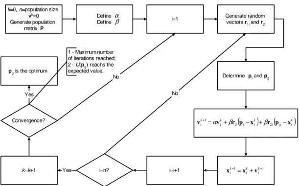
Particle Swarm
Another evolutionary method is the one that uses the concepts of Particle Swarm. Such method was created in 1995 by an Electrical Engineer (Russel Eberhart) and a Social Psychologist (James Kennedy) (Kennedy and Eberhart, 1995; Kennedy, 1999; Naka et al, 2001; Eberhart et al, 2001) as an alternative to the Genetic Algorithm Method. This method is based on the social behavior of various species and tries to equilibrate the individuality and sociability of the individuals in order to locate the optimum of interest. The original idea of Kennedy and Eberhart came from the observation of birds looking for nesting places. When the individuality is increased, the search for alternative places for nesting is also increased. However, if the individuality becomes too high, the individual might never finds the best place. On the other hand, when the sociability is increased, the individual learns more from its neighbors’ experience. However, if the sociability becomes too high, all the individuals might converge to the first minima found, which is possibly a local minima.
In this method, the iterative procedure is given by:
1 1
v x x+ = + ki+
k i k
i (29.a)
(
) (
k)
i g i k i i i k i k
i v r p x r p x
v 1 2
1= + − + −
+ α β β (29.b)
where:
xi is the i-th individual vector of parameters.
vi = 0, for k=0.
r1i and r2i are random numbers with uniform distribution
between 0 and 1.
pi is the best value found for the vector xi.
pg is the best value found for the entire population.
0 < α < 1; 1 < β < 2
In Eq. (29.b), the second term on the right hand side represents the individuality and the third term the sociability. The first term on the right-hand side represents the inertia of the particles and, in general, must be decreased as the iterative process runs. In this equation, the vector pi represents the best value ever found for the
i-th component vector of parameters xi during the iterative process.
Thus, the individuality term involves the comparison between the current value of the i-th individual xi with its best value in the past.
The vector pg is the best value ever found for the entire population
of parameters (not only the i-th individual). Thus the sociability term compares xi with the best value of the entire population in the
past.
k=0, n=population size
vk=0
Generate population matrix P
Generate random vectors r1i and r2i Define
Define
k=k+1
Convergence? pg is the optimum
Yes
No 1 - Maximum number of iterations reached; 2 - U(pg) reachs the expected value.
α β
(
)
(
k)
i g i k i i i k i k
i v r p x r p x
v+ = + 1 − + 2 −
1 α β β
1
1 +
+ = + k
i k i k
i x v
x
Determine pi and pg i=1
i=n? i=i+1
Yes
No
Figure 6. Iterative procedure for the Particle Swarm Method.
Simulated Annealing
This method is based on the thermodynamics of the cooling of a material from a liquid to a solid phase (Corana et al, 1987; Goffe et al, 1994). If a liquid material (e.g. liquid metal) starts being slowly cooled down and left for a sufficiently long time close to the phase change temperature, a perfect crystal will be created, which has the lowest internal energy state. On the other hand, if the liquid material is not left for a sufficient long time close to the phase change temperature, or, if the cooling process is not sufficiently slow, the final crystal will have several defects and a high internal energy state. This is similar to the quenching process used in metallurgical applications.
We can say that gradient-based methods “cool down too fast”, going rapidly to an optimum location which, in most cases, is not the global but the local one. Differently from the gradient-based methods, the Simulated Annealing Method can move in any direction, escaping from possible local minimum or maximum values. Consider, for example, the Boltzmann probability function
( )
(E KT) eE /
Prob ∝ − (30)
This equation expresses the idea that a system in thermal equilibrium has its energy distributed probabilistically among different energy states E. In this equation, K is the Boltzmann constant. Such equation tells us that, even at low temperatures, there is a chance, even small, that the system is at a high energy level, as
illustrated in Fig. 7. Thus, there is a chance of the system to get out of this local minimum and search for a global one.
E/kT
P
ro
b
(
E
)
Low temperature Small Probability of high energy state
High temperature High Probability of high energy state
Figure 7. Schematic representation of Eq. (30).
Figure 8 shows the iterative procedure for the Simulated Annealing Method. The procedure starts by generating a population of individuals of the same size of the number of variables (n=m), in such a way that the population matrix is a square matrix. Then, the initial temperature (T), the reducing ratio (RT), the number of cycles (Ns) and the number of iterations of the annealing process (Nit) are
selected. After NSn function evaluations, each element of the step
length V is adjusted, so that approximately half of all function evaluations are accepted. The suggested value for the number of cycles is 20. After NitNsn function evaluations, the temperature (T) is
m=number of variables n=population size=m Make a initial guess for
x=x0 and U(x0)
i=i+1 Define initial
temperature T; temperature reducing
ration RT; number of cycles Ns; number of iterations Nit
xi
0=x i 1 Objective function
goes dow n
Convergence?
Calculate
Yes No
1 - Maximum number of iterations reached; 2 - U(xk) reachs the expected value.
i i i x RV
x1= 0+
Calculate U(xi 1) Generate a random
number R i=0; j=0; k=0
Ni=0, w here i=1,...,m
U(xi
1)<U(x i 0)?
Yes No
Ni=Ni+1 ( ) ( )
[Uxi Uxi]T
e P 1− 0/
=
Generate a random number R
P<R?
Yes No
xi
0=x i 1 Objective function
goes up Reject xi
1
i=m?
Yes
No
A
Goto
A
j=j+1 j=Ns?
Yes
No Goto
A
Calculate
s i N
N r= /
r>0.6?
Yes No
( )
+ −
=
4 . 0
6 . 0 2
1 r
V Vi i
( )
+ −
=
4 . 0
4 . 0 2
1 r
V Vi i
k=k+1 k=Nit?
Yes
No
Goto
A
Reduce the temperature T=T*RT
Goto
B
B
xk is the optimum
Figure 8. Iterative procedure for the Simulated Annealing Method.
The iterative process is given by the following equation:
i i i x RV
x1= 0+ (31)
where R is a random number with uniform distribution between 0 and 1 and V is a step-size which is continuously adjusted.
To start, it randomly chooses a trial point within the step length
V (a vector of length N) of the user selected starting point. The
function is evaluated at this trial point (xi1) and its value is compared
to its value at the initial point (xi0). In a minimization problem, all
downhill moves are accepted and the algorithm continues from that trial point. Uphill moves may be accepted; the decision is made by the Metropolis criteria. It uses T (temperature) and the size of the downhill move in a probabilistic manner
( ) ( )
[
Uxi Uxi]
Te
P= 1− 0 / (32)
The smaller T and the size of the uphill move are, the more likely that move will be accepted. If the trial is accepted, the algorithm moves on from that point. If it is rejected, another point is chosen for a trial evaluation.
Each element of V is periodically adjusted, so that half of all function evaluations in that direction are accepted. The number of accepted function evaluations is represented by the variable Ni. Thus the variable r represents the ratio of accepted over total function evaluations for an entire cycle Ns and it is used to adjust the step
A decrease in T is imposed upon the system with the RT variable by using
) ( * ) 1
(i RT Ti
T + = (33)
where i is the i-th iteration. Thus, as T declines, uphill moves are less likely to be accepted and the percentage of rejections rises. Given the scheme for the selection for V, V falls. Thus, as T declines, V falls and the algorithm focuses upon the most promising area for optimization.
The parameter T is crucial for the successful use of the algorithm. It influences V, the step length over which the algorithm searches for the minimum. For a small initial T, the step length may be too small; thus not enough values of the function will be evaluated to find the global minimum. To determine the starting temperature that is consistent with optimizing a function, it is worthwhile to run a trial run first. The user should set RT = 1.5 and
T = 1.0. With RT > 1.0, the temperature increases and V rises as
well. Then the T must be selected that produces a large enough V.
Hybrid Methods
The so-called Hybrid Methods are a combination of the deterministic and the evolutionary/stochastic methods, in a sense that the advantages of each one of them are used. Hybrid Methods usually employ an evolutionary/stochastic method to locate the region where the global minimum is located and then switches to a deterministic method to get closer to the exact point faster.
As an example, consider the Hybrid Method illustrated in Fig. 9. The main module is the Particle Swarm Method, which does almost the entire optimization task. When some percentile of the particles find a minima (let us say, some birds already found their best nesting place), the algorithm switches to the Differential Evolution Method and the particles (birds) are forced to breed. If there is an improvement of the objective function, the algorithm returns to the Particle Swarm Method, meaning that some other region is more prone to have a global minimum. If there is no improvement of the objective function, this can indicate that this region already contains the global minimum expected and the algorithm switches to the BFGS Method in order to locate more precisely its location. Finally, the algorithm returns again to the Particle Swarm Method in order to check if there are any changes in the minimum location and the entire procedure is repeated for a few more iterations (e.g., 5).
More involved Hybrid Methods, dealing with the application of other deterministic and stochastic methods, can be found in references (Colaço et al, 2003a; Colaço et al, 2004; Colaço et al, 2003b; Dulikravich et al, 2003a; Dulikravich et al, 2003b; Dulikravich et al, 2003c; Dulikravich et al, 2004; Colaço et al, 2003c).
Particle Swarm using Boltzmann
probability
Differential Evolution
m% of the particles found a minima
Improvement of the objective function
No-improvement of the objective function
Function Estimation Approach
The methods described above were applied for the minimization of an objective function U(x), where x = [x1, x2, … , xN] is the vector with the parameters of the problem under consideration that can be modified in order to find the minimum of U(x). Therefore, the minimization is performed in a parameter space of dimension N. Several optimization or inverse problems rely on functions, instead of parameters, which need to be selected for the minimization of an objective function. In these cases, the minimization needs to be performed in an infinite dimensional space of functions and no a
priori assumption is required regarding the functional form of the
unknown functions, except for the functional space that they belong to (Alifanov, 1994; Alifanov et al, 1995; Ozisik and Orlande, 2000). A common selection is the Hilbert space of square integrable functions in the domain of interest.
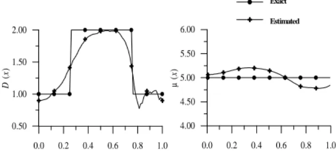
In this paper we use the conjugate gradient method with adjoint problem formulation for the minimization of the objective function. We illustrate here the function estimation approach as applied to the solution of a specific inverse problem involving the following diffusion equation (Colaço et al, 2003c):
* *) r ( * *] *) r ( * [ *
*) *, r ( * *) r (
* D T T
t t T
C =∇⋅ ∇ +µ
∂
∂ (34)
where r* denotes the vector of coordinates and the superscript * denotes dimensional quantities.
Equation (34) can be used for the modeling of several physical phenomena, such as heat conduction, groundwater flow and tomography. We focus our attention here to a one-dimensional version of Eq. (34) written in dimensionless form as
( ) + ( ) in 0< <1,for >0
∂ ∂ ∂
∂ = ∂ ∂
t x T x x T x D x t
T µ (35.a)
and subject to the following boundary and initial conditions.
0
= ∂ ∂ x
T at x=0 for t>0 (35.b)
( )
=1∂ ∂ x T x
D at x=1 for t>0 (35.c)
0
=
T for t=0 in 0<x<1 (35.d) Notice that in the direct problem, the diffusion coefficient function D(x) and the source term distribution function µ(x) are regarded as known quantities, so that a direct (analysis) problem is concerned with the computation of T(x,t).
Inverse Problem