Raul Guenther
Member, ABCM [email protected] Depto. Engenharia Mecânica Universidade Federal de Santa Catarina- 88040-900 Florianópolis, SC, Brazil
Eduardo C. Perondi
[email protected] Universidade Federal do Rio Grande do Sul Rua Sarmento Leite 425 90050-170 Porto Alegre, RS, BrazilEdson R. DePieri
[email protected] Depto. de Automação e Sistemas Universidade Federal de Santa Catarina 88040-900 Florianópolis, SC, BrazilAntônio C. Valdiero
valdiero@unijuí.tche.brUNIIJUÍ 98280-000 Panambi, RS, Brazil
Cascade Controlled Pneumatic
Positioning System with LuGre Model
Based Friction Compensation
This paper proposes a cascade controller with friction compensation based on the LuGre model. This control is applied to a pneumatic positioning system. The cascade methodology consists of dividing the pneumatic positioning system model into two subsystems: a mechanical subsystem and a pneumatic subsystem. This division allows the introduction of friction compensation at force level in the pneumatic positioning system. Using Lyapunov´s direct method, the convergence of the tracking errors is shown under the assumption that the system parameters are known. Experimental results illustrate the main characteristics of the proposed controller.
Keywords: Servopneumatics, robotics, cascade control, friction compensation
Introduction
Pneumatic positioning systems are very attractive for many applications because they are cheap, lightweight, clean, easy to assemble and present a good force/weight ratio. In spite of these advantages, pneumatic positioning systems possess some undesirable characteristics which limit their use in applications that require a fast and precise response. These undesirable characteristics derive from the high compressibility of the air and from the nonlinearities present in pneumatic systems.1
To overcome the difficulties introduced by the high compressibility of the air and by the nonlinear air flow through the servovalve, a cascade control strategy has been developed in which the pneumatic positioning system is interpreted as an interconnected system: a mechanical subsystem driven by the force generated by a pneumatic subsystem (Guenther and Perondi, 2002).
Nonlinear friction is another important factor that affects the precision of the system position response. In pneumatic positioning systems the friction forces between the slider-piston system surfaces in contact are strongly dependent on the physical characteristics of the contacting surfaces, such as their material properties and geometry, and their lubrication conditions.
Classical friction models use static mappings that describe the steady state relation between velocity and friction force, which can be characterized by the viscous and Coulomb friction with Stribeck effect combination. However, some friction phenomena cannot be captured by static mapping, as for example, hysteretic behaviour with non-stationary velocity and breakaway force variations. Therefore, in the mechanics-related controller design, simple classical models are not sufficient to address applications with high-precision positioning requirements and low velocity tracking. Thus, to obtain accurate friction compensation and best control
Paper accepted September, 2005. Technical Editor: Atila P. Silva Freire.
performance, friction forces model with dynamic behaviour is necessary (Armstrong et al., 1994).
A friction model that represents most of the steady state and dynamic friction properties, the LuGre model, has been proposed by Canudas de Wit et al. (1995). In this model, the friction force is modelled as the average deflection force of elastic bristles between two contacting surfaces. The tangential force applied to the contacting objects causes the bristles to deflect like springs. The average deflection is modelled by a first-order nonlinear differential equation, which describes the dynamic behaviour of the overall friction force.
Although friction compensation is especially important for pneumatic devices, it is particularly difficult to be performed using non-model based compensation or even model-based compensation (see Armstrong et al., 1994). The model-based friction compensation, adopted in this work, uses an on-line friction force estimation scheme. The compensation is achieved by adding the estimated friction force to the reference force generated by the position controller at the force level. To use this compensation scheme it is usually assumed that the actuator has a fast and accurate force response (Canudas de Wit et al., 1995, Lischinsky et al., 1999). This assumption is generally verified for positioning systems with electric actuators and sometimes for positioning systems with hydraulic actuators. Nevertheless, most pneumatic positioning systems do not provide a sufficiently fast and efficient force response.
Wit et al. (1995) requires slight modifications to be applied in the cascade control scheme.
This paper presents a cascade controller scheme that applies the LuGre model friction compensation technique to a pneumatic positioning system. The convergence of the tracking errors is demonstrated using the Lyapunov direct method when all the system parameters are known and there are no external forces. Experimental results illustrate the main properties of the proposed controller.
This paper is organized as follows. In Section 2, the experimental test rig is described. Section 3 is dedicated to the presentation of the theoretical model of the investigated system, while, in Section 4, the cascade controller and the proposed friction force estimator are described. The controller stability properties are stated in Section 5. In Section 6, the experimental results are presented. Finally, the main conclusions are outlined in Section 7.
Nomenclature
A = piston area, m2
cp = air specific heat at constant pressure, J/Kg K
cv = air specific heat at constant volume, J/Kg K
d(t) = disturbance
D = tracking error matrix
e(t) = error function F = force, N Fa = friction force, N
Fc = Coulomb friction force, N
Fe = external forces, N
Fs = static friction force, N
g = continuous vector force, N
g(t) = action force, N gd(t) = desired action force, N
H(s) = generic transfer function
hˆ = pneumatic subsystem dynamics independent of the control voltage
I = identity matrix K = positive gain
KD = cascade controller’s positive gain
Ko = positive gain
KP = cascade controller’s positive pressure gain
kv = real positive constant
L = piston stroke, m M = mass, Kg
m(.) = smoothing function
N = state dependent matrix p = absolute pressure, Pa p∆ = pressure drop, Pa P = real positive constant P∆δ = desired pressure drop, Pa Q = heat transfer energy, J qm = mass flow rate, Kg/s
QN = nominal volumetric flow rate[m3/s]
R = gas constant, KgJ/K
R = residual set
r = specific heat ratio, dimensionless s = velocity error function, m/s s = Laplace operator
T = temperature, K t = time, s
u = control voltage signal, V ua = auxiliary signal
*
a
u = ideal auxiliary signal
û = pneumatic subsystem dynamics dependent of the control voltage, m3/s
V10 = fixed volume at chamber 1 end of the stroke, m3
V20 = fixed volume at chamber 2 end of the stroke, m3
V = non negative scalar function, Lyapunov´s function y(t) = piston position, m
yd(t) = desired piston position, m
máx
y = extreme desired position, m
r
y = reference velocity, m/s
s
y = threshold Stribeck velocity, m/s z = presliding displacement Greek Symbols
γ = maximum/minimum eigenvalue ratio, bounded real number
η = constant that measures trajectory speed
λ = cascade controller’s gain
λmax = maximum eigenvalue
λmin = minimum eigenvalue
ρ = density [Kg/m3]
ρρρρ = closed loop tracking error
σ0 = elastic stiffness coefficient [N/m 2
]
σ0e = estimated elastic stiffness coefficient [N/m 2
]
σ1 = friction coefficient [Ns/m]
σ2 = viscous friction coefficient [Ns/m]
ω = frequency [rad/s]
Ω = a specific domain
ϖn = natural frequency [rad/s]
ζ = dumping ratio, dimensionless Subscripts
*
relative to exact or known value
0 relative to initial or normalized conditions 1 relative to cylinder’s chamber 1
2 relative to cylinder’s chamber 2 d relative to desired condition I relative to initial condition
max relative to maximum value condition min relative to minimum value condition N relative to nominal value
r relative to reference signal
∆ relative to gradient
The Pneumatic Positioning System
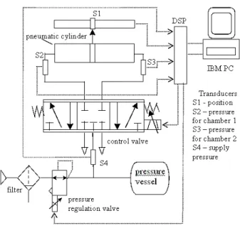
The system under consideration is shown in Fig.1. It consists of a proportional servovalve 5/3 (MPYE-5-1/8 FESTO) that drives a double action rodless cylinder, with internal diameter of 0.025 [m] and 1 [m] stroke (DGPL-1000 FESTO).
The measured nominal flow rate is QN = 7.10-3 [m3/s] (420
Figure 1. Experimental rig.
The Dynamic Model
The dynamic model used in this work is developed based on: (i) the description of the relationship between the air mass flow rate and pressure changes in the cylinder chambers, and (ii) the equilibrium of the forces acting at the piston, including the friction force.
The relationship between the air mass flow rate and the pressure changes in the chambers is obtained using energy conservation laws, and the force equilibrium is given by Newton’s second law. The friction force is included in the LuGre friction model.
Conservation of Energy
The internal energy of the mass flowing into chamber 1 is T
q
Cp m1 , where Cp is the constant pressure specific heat of the air,
T is the air supply temperature, and qm1=
(
dm1 dt)
is the air massflow rate into chamber 1. The rate at which work is done by the moving piston is p1V1, where p1 is the absolute pressure in
chamber 1 and V1=
(
dV1 dt)
is the volumetric flow rate. The timeair internal energy change rate in the cylinder is d
(
CVρ1V1T)
dt,where CV is the constant volume specific heat of the air and ρ1 is the
air density. We consider the ratio between the specific heat values as
V P C C
r= and that ρ1=CV (RT) for an ideal gas, where R is the universal gas constant. An energy balance yields
) ( 1
1 1 1
1
1 pV
dt d rR dt dV C
p T q
P
m − = (1)
where the rate of heat transfer through the cylinder walls ( Q ) is considered negligible. The total volume of chamber 1 is given by
10 1 Ay V
V = + , where A is the cylinder cross-sectional area, y is the piston position and V is the dead volume of air in the line and at 10 the chamber 1 extremity. The change rate for this volume is
y A
V1= , where y=dy/dt is the piston velocity. After calculating
the derivative term in the right hand side of (1) we can solve this equation to obtain
1
10 1
10
1 qm
V Ay
RrT p V Ay
y Ar p
+ + + −
= (2)
where Cp=(rR)/(r−1).
Similarly for chamber 2 of the cylinder we obtain
2 20 2
20 2
) ( )
( AL y V qm
RrT p
V y L A
y Ar p
+ − + + −
= (3)
where L is the cylinder stroke.
Assuming that the mass flow rates are nonlinear functions of the servovalve control voltage (u) and of the cylinder pressures, that is,
) , ( 1
1 1 q p u
qm = m and qm2=qm2(p2,u), expressions (2) and (3) result in
) , ( 1
1 10 1
10
1 q p u
V Ay
RrT p V Ay
y Ar
p m
+ + + −
= (4)
) , ( )
( )
( 20 2 2
2 20
2 q p u
V y L A
RrT p
V y L A
y Ar
p = − + + − + m (5)
Piston Dynamics
Applying Newton’s second law to the piston-load assembly results in
) (p1 p2 A F F y
M + a+ e= − (6)
where M is the mass of the piston-load assembly, Fa is the friction force, Fe is the external force and A(p1−p2) is the force related to the pressure difference between the two sides of the piston (see Fig. 2).
Figure 2. Force equilibrium at the piston.
Friction Model
In this paper the friction force (F ) is described according to the a LuGre friction model proposed by Canudas et al. in [2]. This model satisfies the requirements for friction compensation in pneumatic systems because it can describe complex friction behavior, such as stick-slip motion, presliding displacement, Dahl and Stribeck effects and frictional lag.
In this model the friction force is given by
y dt dz z
Fa=σ0 +σ1 +σ2 (7)
where z is a friction internal state that describes the average elastic deflection of the contact surfaces during the stiction phases, the parameter σ0 is the stiffness coefficient of the microscopic
2
m q
1
m q
) (p1 p2
A −
M y
y y, ,
Fa
Fe
chamber 1 chamber 2
2
p
1
deformations z during the presliding displacement, σ1 is a damping
coefficient associated with dzdt and σ2 represents the viscous friction. The dynamics of the internal state z are expressed by
z y g y y dt dz ) ( 0 σ − = (8)
where g(y) is a positive function that describes the “steady-state” characteristics of the model for constant velocity motions and is given by 2 ) ( ) ( )
( y ys
c s
c F F e
F y
g = + − − (9)
where F is the Coulomb friction force, C F is the static friction S
force and y is the Stribeck velocity. In equation (9) it can be S observed that g( y) is bounded by the static friction force F . s
An important property of the LuGre friction model is that the average elastic deflection z is bounded. This statement can be outlined by considering the following Lyapunov candidate function:
2 2 1z
V = (10)
Differentiating (10) and combining with equation (8), it can be written: ⋅ − ⋅ ⋅ ⋅ −
= sign(y) sign(z) ) y ( g z z y dt
dV σ0
(11)
The time derivative of the Lyapunov candidate function dV/dt given in (11) is negative if |z>g
( )
y/σ0, since g( )
y is strictlypositive and bounded by Fs (see equation (9)). It results that the set
Π= { z: |z| ≤ Fs /σ0 } is an invariant set for the solutions of equation
(8), and that the elastic deflection z is bounded.
The Interconnected Model
Equations (4), (5), (6), (7) and (8) constitute a fifth order nonlinear dynamic model of the pneumatic positioning system with friction. To rewrite this model in an interconnected form, appropriate for our cascade controller design, we define
∆
= +
+F F Ap
y
M a e (12)
The pressure difference change rate, calculated using expressions (4) and (5), is given by
+ − − + = ∆ 20 2 2 10 1 1 ) ( ) , ( ) , ( V y L A u p q V Ay u p q RrT
p m m
+ − + + − 20 2 10 1 ) (L y V A p V Ay p y rA (13)
Separating p into the terms affected by the servovalve control ∆
voltage u and the terms which are functions only of piston position and velocity, we obtain the functions uˆ=uˆ(p1,p2,y,u)and
) , , , ( ˆ ˆ 2 1 p y y
p h
h= , given, respectively, by
+ − − + = 20 2 2 10 1 1 2 1 ) ( ) , ( ) , ( ) , , , ( ˆ V y L A u p q V Ay u p q RrT u y p p
u m m
(14) + − + + − = 20 2 10 1 2 1 ) ( ) , , , ( ˆ V y L A p V Ay p y rA y y p p h (15)
This allows us to rewrite expression (13) as
) , , , ( ˆ ) , , , ( ˆ 2 1 2
1 p y y u p p yu
p h
p∆ = + (16)
Equations (12) and (16) describe the pneumatic positioning system dynamics.
y
y
u p∆
Pneumatic positioning system
pneumatic subsystem
mechanical subsystem
Figure 3. Pneumatic system described as two interconnected subsystems.
Equation (12) represents the mechanical subsystem driven by a pneumatic force g=Ap∆. Equation (16) describes the dynamics of
the pneumatic subsystem in which this pneumatic force is generated by commanding the control voltage u appropriately. This interpretation reinforces the interconnected model description (Fig.3).
The Cascade Control Strategy
We present here the cascade control strategy based on the methodology of order reduction described in Utkin (1987). This cascade control strategy has been used successfully in the control of robot manipulators with electric actuators (Guenther and Hsu, 1993), to control flexible joint manipulators (Hsu and Guenther, 1993) and hydraulic actuators (Guenther and De Pieri, 1997, Cunha et al., 2002).
According to this strategy, the pneumatic positioning system is interpreted as an interconnected system like that presented in Fig.3 and its equations can thus be rewritten in a convenient form. To perform this task we initially define the pressure difference tracking error as
d
p p p∆ = ∆− ∆
~ (17)
where p∆d is the desired pressure difference to be defined based on
the desired force gd =Ap∆d. This is the desired force required on
the piston-load assembly mass to obtain a desired tracking performance. Using the definition (17), equations (12) and (16) may be rewritten as
My=Ap∆d+d(t) (18)
) , , , ( ˆ ) , , , ( ˆ 2 1 2
1 p y y u p p yu
p h
p∆ = + (19)
e
a F
F p A t
d()= ~∆− − (20)
The system (18)(19) is in the cascade form. Equation (18) can be interpreted as a mechanical subsystem driven by a desired force
d
d Ap
g = ∆ and subjected to an input disturbance d(t). Equation
(19) represents the pneumatic subsystem.
The design of the cascade controller for the system (18)(19) can be summarized as follows:
(i) – Compute a control law gd(t)=Ap∆d(t) for the mechanical subsystem (18) such that the piston displacement (y(t)) achieves a desired trajectory yd(t) taking into account the presence of the disturbance d(t); and then
(ii) – Compute a control law u(t) such that the pneumatic subsystem (19) applies a pneumatic force g(t)=Ap∆(t) to the mechanical subsystem that tracks the desired force gd(t)=Ap∆d(t). In this paper the design of the mechanical subsystem control law gd(t) is based on the controller proposed by Slotine and Li (1988), including a friction compensation scheme based on the LuGre friction model. The control law u(t) is synthesized to achieve good tracking performance characteristics related to the pneumatic subsystem.
Friction Force Observer
According to Canudas de Wit et al. (1995) the estimated friction
force Fˆ is given by a
y dt
z d z
Fa 0 1 2
ˆ ˆ
ˆ =σ +σ +σ (21)
where zˆ t() is the estimated friction internal state given by
y K z y g
y y dt
z
d ~
ˆ ) ( ˆ
0 0 −
−
= σ (22)
and K is a positive constant. 0
In Canudas de Wit et al. (1995) the authors show that the friction force observer (21)(22) applied to an electric actuator leads the position error ~ ty() to converge asymptotically to zero if the electric actuator position controller is designed such that the dynamic relating the position error ~ ty() and the estimation error
) ( ˆ ) ( ) (
~t zt z t
z = − is strictly positive real (SPR).
The observer (22) requires a slight modification to be used within the cascade control scheme. This modification is required because the value of the friction force time change rate F is used a to calculate the control signal in the cascade control strategy. So, the function y has to be smoothed by a function m(y) (like
) arctan( ) 2 ( )
(y y ky
m = π v , where k is a positive constant, for v
example). Note that, as with the function y , the function m(y) is
equal to zero at the origin (m(0)=0).
Additionally, to achieve the desired stability properties for the pneumatic positioning system closed loop, it is proposed in this paper that the internal state zˆ t() is estimated using the following modified observer
Ks z y g
y m y dt
z d
0 0 ˆ
) (
) ( ˆ
σ
σ −
−
= (23)
where K is a positive constant and s is the measure of the velocity tracking error defined in equation (27).
Introducing the function m( y), the residual difference 0
) ( ≥
∆ y is defined as
∆(y)= y−m(y) (24)
and the friction internal state estimating error ~ tz() is given by
Ks z y g
y z y g
y m dt
z d
0 0 0
) (
) ( ~ ) (
) ( ~
σ σ
σ −∆ +
−
= (25)
Tracking Control of the Mechanical Subsystem
Based on Slotine and Li (1988) and including the friction compensation, the following control law to obtain trajectory tracking in the mechanical subsystem is proposed:
a D r
d My K s F
g = − + ˆ (26)
where K is a positive constant, D y is the reference velocity and s r
is a measure of the velocity tracking error.
In fact, y can be obtained by modifying the desired velocity r y as d
follows
y y
yr= d−λ~ ; ~y=y−yd; s=y−yr =~y+λ~y (27)
where λ is a positive constant.
Let the friction force be given according to the LuGre friction model (7). Substituting (26) in (18) and using definition (20) and the observer (21)(23), the error equation related to the mechanical subsystem becomes
e
Ds z z Ap F
K s
M + +σ1~+σ0~= ~∆− (28)
Consider the non-negative function
2 1 2 1
~
2V =Ms +K−z (29)
Using (25) and (28), the time derivative of (29) along the mechanical subsystem trajectories is given by
z s y g
y m z y g
K y m s p A s K K
V D
~ ) ( ) ( ~ ) ( ) ( ~ )
( 2 0 1
1 0 2
0 1 1
σ σ σ
σ
σ + − +
+ −
= ∆ −
z z y g
y K s F zs y g
y
e
~ ) (
) ( )
( )
( 1 0
1
0 ∆ − − ∆
+σσ − σ (30)
Expression (30) will be used in the stability analysis.
Tracking Control of the Pneumatic Subsystem
In order to obtain force tracking in the pneumatic subsystem (19) we propose the following control law
As p K u
where u is an auxiliary control signal, a K is a positive constant, A P
is the cylinder cross-sectional area, and s is defined in (27).
Substituting (31) in (19), the resulting pneumatic subsystem closed loop dynamics gives
As p K u y y p p h
p∆= ˆ( 1, 2, , )+ a− p~∆− (32)
The designs of the auxiliary signal u and of the constant a K P
are based on the non-negative function V defined as 2
2 2
~
2V =p∆ (33)
The time derivative of (33) is given by V2= ~p∆(p∆−p∆d), where the time derivative of the desired pressure difference (p∆d =gd/A) is obtained using (26). So, in order to calculate p∆d,
we need to know the acceleration signal. In the ideal case (where all the parameters are known and there is no friction or external forces), the acceleration may be calculated using expression (6) by means of the pressure difference p measurement. ∆
The time derivative of (33) along the pneumatic subsystem trajectories is obtained using the closed loop dynamics (32):
] ~ ˆ
[ ~
2 p u h p K p As
V = ∆ a+ − ∆d− P ∆− (34)
Defining the ideal auxiliary signal as
u*a=p∆d−hˆ(p1,p2,y,y) (35)
results in
] ~ [
~
2 p u K p As
V = ∆ ∆ a− P ∆ − (36)
where *
a a
a u u
u = −
∆ is the auxiliary signal error. In the ideal case,
*
a
a u
u = , ∆ua=0, and expression (36) results in
∆ ∆−
−
= K p Asp
V P
~ ~2
2 (37)
Expression (37) will also be used in the stability analysis.
The Pneumatic Positioning System Controller
The pneumatic positioning system cascade controller is a combination of the mechanical subsystem position tracking control law (26) and the control signal designed to obtain the pneumatic subsystem tracking force (31).
Using (26) we calculate the desired pressure difference to obtain the trajectory tracking in the mechanical subsystem, p∆d=gd A.
In the ideal case, in which *
a
a u
u = , the signal uˆ is calculated using equations (31) and (35). The necessary time derivative of the desired pressure difference is obtained as described above, and the
function hˆ=hˆ(p1,p2,y,y) as defined in (15).
The servovalve control voltage u is obtained through the inverse of the function (14), that is,
) ˆ , , , (p1 p2 yu
u
u= (38)
The use of the inverse defined in (38) and the function
) , , , ( ˆ ˆ 2 1 p y y
p h
h= in the control law may be interpreted as a feedback linearization scheme (see Khalil, 1996).
Stability Analysis
Consider the cascade controlled pneumatic positioning system with the friction observer. In this case the closed loop system is
)} 31 ( ), 26 ( ), 23 ( ), 21 ( ), 16 ( ), 12 {( = Ω .
We assume that the desired piston position yd(t) and its derivatives, up to 3rd order are uniformly bounded.
For the ideal case, in which all the system parameters are known and there is no external forceF , the tracking errors convergence e
properties are stated below.
Theorem – When all the system parameters are known and there is no external forceF , given an initial condition, the controller gains e
can be chosen in order to obtain the convergence of the tracking
errors, ~ ty()and~ ty(), to a residual set R as t→∞. The set R depends on the friction characteristics and the controller gains.
Proof: Consider the lower bounded function
2 1 2 2 2 1 ~ ~ 2 2 ) (
2V t = V + V =Ms +p∆+K−z (39)
where the functions V and 1 V are defined in (29) and (33), 2
respectively.
This expression can be written in the following matrix equation form ρ ρ 1 2 1 N
V = T
(40)
where the error state vector is defined as T
z p
s ~ ~]
[ ∆
=
ρ and N 1
is a positive definite diagonal matrix given by
[
1]
1 1
−
=diagM K
N (41)
In the ideal case ∆ua=0 and, according to the expressions (30) and (37), the time derivative of (39) is given by
2 1 0 2 2 1 0 ~ ) ( ) ( ~ ) ( z y g K y m p K s K K
V D P
− ∆ σ − − σ σ + − = z z y g y K sz y g y z s y g y m ~ ) ( ) ( ) ( ) ( ~ ) ( )
( 0 1 + 0 1∆ − 1 0∆
+ σσ σσ − σ
(42)
Written in a matrix equation form this expression results:
) (
2ρ ρ ρ
ρ N D
V =− T + T
T
z y g
y K z
y g
y D
∆
− ∆
= −
) (
) ( 0
) (
) ( )
(
1 0 1
0σ σ
σ
ρ (45)
The matrix N is state dependent. Specifically it depends on the 2
function g(y) defined in (9) and on the functionm(y), used in order to smooth y in equation (23). In the sequence we establish the conditions to make this matrix be uniformly positive definite.
To this end, first we observe that the function m(y) is equal to zero in the static friction range (y=0), and positive (m(y)>0) if
0 ≠
y .
Out of the static friction range, withy≠0, using the Gershgorin theorem it should be observed that the matrix N in (44) is positive 2 definite if:
i)
( ) ( )
( ) ( )
m y y g ym y g
K1 0 1
0
2 1σσ σ − > −
, and
ii)
( ) ( )
m yy g K
KD
1 0 1
0
2 1σσ σ
σ > −
+ .
From (i) it results that:
1
2 σ <
K (46)
Taken into account that the function m(y) grows as the velocity grows, consider that, given an initial condition, an upper limit to the velocity, ymax, exists. This implies that an upper limit to m(y)
(m(y)≤m∈t>0) also exists.
Since the function g(y) is bounded by the static friction force
S
F , for the given initial condition expression (ii) gives:
−
> K
F m K
S D
2 1
1 0σ
σ (47)
It should be observed that K is a positive constant and so the D following additional restriction should be satisfied:
S
F m K
2 1
< (48)
Under conditions (46), (47) and (48), the matrix N results 2 uniformly positive definite, i.e.:
I
N2≥α (49)
where α is a positive constant given by:
[ ]0, min
( )
2inf N
T
t λ
α= ∈ ∀T ≥0 (50)
Using (49) in (43) and employing the Rayleight-Ritz theorem, it can be written that
) (
2
ρ ρ ρ
α D
V≤− + (51)
Expression (45) allows the observation that the disturbance )
(ρ
D is caused by the bounded elastic deflection z and by the residual difference ∆(y)≥0, defined in (24), which is equal to zero
as the velocity y is null or as y→π 2kv, and is limited otherwise.
So we may establish a superior limit for D(ρ) ≤D. Therefore:
ρ ρ
α D
V≤− 2+ (52)
The condition in which the time derivative V is negative is given by:
α
ρ > D (53)
By the Rayleight-Ritz theorem the expression (40) results
( )
2 1 max 12 1 2
1
ρ λ ρ
ρ N N
V= T <
(54)
Using the condition (53) in (54) allows to verify that the region in which the function V is negative is limited by a constant value. Expressions (52) and (54) show that ρ tends to a residual set as
∞ →
t . Expression (53) outlines that this residual set depends on the value of the disturbance bound D and on the value α defined in (50). Consequently each error vector component tends to a residual. This means that the velocity error measure s(t) tends to a residual set. This error can be interpreted as an input of the first order filter given in (27), and based on this interpretation we conclude that the tracking errors ~ ty() and ~ ty()tend to a residual set as t→∞. This completes the proof.
Remark 1: As ~ ty() tends to a limited residual set, and as the desired velocity yd
( )
t is also limited, from the error definition in (27) it results that the velocity y( )
t is limited, i.e., there is an upper bound ymax as considered above, which depends on the closed loopsystem dynamics and on the initial conditions.
Remark 2: From remark 1 it is clear that the initial conditions should be chosen in order to satisfy the conditions (47) and (48). Therefore, the theorem result depends on the initial conditions, and so, it is a local result.
Remark 3: The “disturbance” upper bound ( D ) depends on the friction characteristics (see (45)) and on the smoothing function
) ( y
m . The positive constant α defined in (50) depends on the controller gains. Therefore, the residual set given by (53) depends on the friction characteristics, on the smoothing function and on the controller gains.
The experimental results presented in the next section validate these theoretical statements.
Experimental Results
The parameters used in the experiments are: A = 4.19x10⁻⁴ [m2], r = 1.4, R = 286.9 [J Kg/K], T = 293.15 [K], L = 1 [m],
=
10
V 1.96x10⁻⁶ [m3], V20= 4.91x10
-6
[m3] and M = 2.9 [Kg]. All experimental tests were realized without applying external forces (F = 0). e
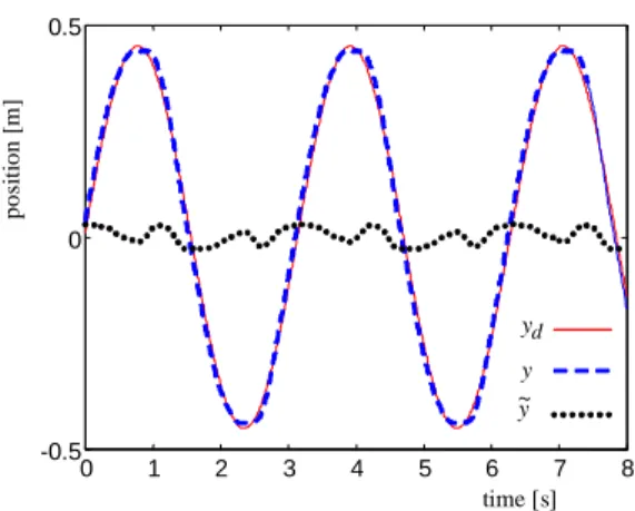
The experimental tests are performed using a sinusoidal and a polynomial desired trajectory. The sinusoidal desired trajectory is given by yd(t)=ymáxsin(wt), ymáx=0,45[m] and w=2 [rad/s] (see Fig. 5a).
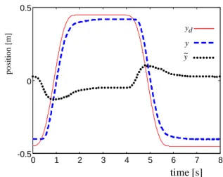
The polynomial trajectory starts with the piston at 0.05 [m] measured from the end of the cylinder (yd(0)=0,05[m]), and reaches a steady-state trajectory at yd(2)=0,95[m] according to a function described by the 7th order polynomial given in (55). This position is maintained for 2 [s]. Then, the piston returns to the initial position in 2 [s] according to a polynomial similar to (55), where it stays for 2 [s], and so on. This desired trajectory is shown in figures 5 and can be described by equations (55) and (56).
4 5 6 7
5 , 10 2 , 25 21 6 )
(t t t t t
ydp =− + − + (55)
The mechanical subsystem controller is designed according to Eq. (26) using equations (21) and (23). The pneumatic subsystem controller is given by Eq. (31), and by the calculation of the auxiliary signal u through Eq. (35), as in the ideal case (a ua=u*a).
] m [
= ) (t
yd 0.05+ydp(t/2) t<2 95
.
0 2≥t<4 )
2 / ) 4 (( 95 .
0 −ydp t− 4≥t<6
05 .
0 6≥t<8 (56)
In order to obtain a response without actuator vibrations and a sufficiently smooth control signal, the control gains are chosen as
= D
K 40, λ=20, KP =150, and the friction force observer parameters are σ0= 4500, σ1= 93.13, σ2= 89.86, v = 0.02 [m/s], s
c
F =32.9 [N], F =38.5 [N], s K =2.22x10⁻⁶.
In the experimental implementation, the velocity is obtained using a filter and a numeric derivative process and the acceleration is calculated based on the nominal parameters.
Figure 4 presents the polynomial desired trajectory, the response to this trajectory using the cascade controller with friction compensation and the tracking error obtained in this case. In order to outline the friction compensation effect, Fig.5 shows the response obtained without this compensation and the respective tracking error. The tracking errors for both cases are presented in detail in Fig. 6. while Fig. 7 shows the control signal using friction compensation.
0 1 2 3 4 5 6 7 8
-0.5 0 0.5
time [s]
p
o
si
ti
o
n
[
m
]
yd
y
y~
Figure 4. Polynomial y,yd and ~y trajectories with friction compensation.
0 1 2 3 4 5 6 7 8
-0.5 0 0.5
time [s]
p
o
si
ti
o
n
[
m
]
yd
y
y~
Figure 5. Polynomial y,yd and ~ytrajectories without friction compensation.
The results presented in Figures 4, 5, 6 and 7 outline the efficiency of the proposed friction compensation in diminishing the trajectory tracking errors and the steady state position error. These experimental results confirm the tracking error convergence theoretically established.
0 1 2 3 4 5 6 7 8
-0.2 -0.15 -0.1 -0.05 0 0.05 0.1 0.15
time [s]
p
o
si
ti
o
n
e
rr
o
r
[m
]
with compensation without compensation
Figure 6. Polynomial tracking position error for both cases.
0 1 2 3 4 5 6 7 8
-0.2 -0.1 0 0.1 0.2 0.3
time [s]
co
n
tr
o
l
si
g
n
al
[V
]
0 1 2 3 4 5 6 7 8 -0.5
0 0.5
time [s]
p
o
si
ti
o
n
[
m
]
yd
y
y~
Figure 8. Sinusoidal y,yd and y~trajectories with friction.
Figure 8 presents the desired sinusoidal trajectory, the response to this trajectory using the cascade controller with friction compensation and the tracking error obtained in this case. Figure 9 shows the response obtained without this compensation and the respective tracking error.
0 1 2 3 4 5 6 7 8
-0.5 0 0.5
time [s]
p
o
si
ti
o
n
[
m
]
yd
y
~y
Figure 9. Sinusoidal y,yd and y~trajectories without friction compensation.
The tracking errors for both cases are presented in detail in Fig. 10. Figure 11 shows the control signal using friction compensation. These experimental results confirm the importance of the friction compensation.
Conclusions
In this work a cascade controller with friction compensation for a pneumatic positioning system was proposed, and the convergence of its tracking errors was theoretically and experimentally demonstrated. It was outlined that the cascade control strategy allows the use of the LuGre friction model without any assumptions about the force response in the actuator. The experimental results confirm the theoretical results and demonstrate the efficiency of the friction compensation. Future research will include methods to deal with the system parameter uncertainties.
0 1 2 3 4 5 6 7 8
-0.2 -0.15 -0.1 -0.05 0 0.05 0.1 0.15
with compensation without compensation
time [s]
p
o
si
ti
o
n
e
rr
o
r
[m
]
Figure 10. Sinusoidal tracking position error for both cases.
0 1 2 3 4 5 6 7 8
-0.2 -0.1 0 0.1 0.2 0.3
time [s]
c
o
n
tr
o
l
si
g
n
al
[
V
]
Figure 11. Control signal u (with friction compensation).
Acknowledgements
This work has the financial support of Brazilian government agency CNPq (Conselho Nacional de Desenvolvimento Científico e Tecnológico.
References
Armstrong-Hélouvry, B., Dupont P. and Canudas de Wit, C., 1994, “A Survey of Models, Analysis Tools, and Compensation Methods for Control of Machines with Friction”, Automatica, Vol. 30, n. 7, pp.1083-1138.
Canudas de Wit, C., Olsson, H., Astrom, K.J. and Lischinsky, P., 1995, “A New Model for Control Systems with Friction”, IEEE Transactions on Automatic Control, Vol. 40, n.3, pp.419-425.
Guenther, R. and Hsu, L., 1993, “Variable Structure Adaptive Cascade Control of Rigid-Link Electrically Driven Robot Manipulators”, Proc. IEEE 32nd CDC Conference on Decision and Control, San Antonio, Texas, USA, pp.2137-2142.
Guenther, R. and De Pieri, E.R.,1997, “Cascade Control of the Hydraulic Actuators”, Revista Brasileira de Ciências Mecânicas, ABCM, Vol. 19, n.2, pp. 108-120.
Guenther R., Cunha, M.A.B., De Pieri, E.R. and De Negri, V.J, 2000, ”VS-ACC Applied to a Hydraulic Actuator”, Proc. of the American Control Conference 2000, Chicago, USA, pp. 4124-4128.
Guenther R. and Perondi, E.A., 2002 , “O Controle em Cascata de um Sistema Pneumático de Posicionamento”, Anais do XIV Congresso Brasileiro de Automática - CBA 2002, Natal, RN, pp.936-942.
Hsu, L. and Guenther, R., 1993 , “Variable Structure Adaptive Cascade Control of Multi-Link Robot Manipulators with Flexible Joints: The Case of Arbitrary Uncertain Flexibilities”, Proc. IEEE Conference in Robotic Automation, Atlanta, Georgia, USA, pp340-345.
Khalil,H. K., 1996, “Nonlinear systems”, 2nd edition, New Jersey, USA,
Lischinsky, P., Canudas de Wit, C. and Morel, G., 1999 , “Friction Compensation for an Industrial Hydraulic Robot”, IEEE Control Systems, pp. 25-32, February.
Perondi E. and Guenther, R.,, 2003, “Modeling of a Pneumatic Positioning System”, Science & Engineering Journal, 01/2003.
Slotine, J-J.E. and Li, W., 1988 , “Adaptive Manipulator Control: A Case Study”, IEEE Transactions on Automatic Control, Vol. 33, n. 11, pp. 995-1003,.