Frederico M. A. Silva
[email protected] Federal University of Goiás Civil Engineering Department 74605-220 Goiânia, Goiás, BrazilPaulo B. Gonçalves
[email protected] Pontifical Catholic University of Rio de Janeiro Civil Engineering Department 22453-900 Rio de Janeiro, RJ, BrazilZenón J. G. N. Del Prado
[email protected] Federal University of Goiás Civil Engineering Department 74605-220 Goiânia, Goiás, BrazilInfluence of Physical and Geometrical
System Parameters Uncertainties on
the Nonlinear Oscillations of
Cylindrical Shells
This work investigates the influence of physical and geometrical system parameters uncertainties and excitation noise on the nonlinear vibrations and stability of simply-supported cylindrical shells. These parameters are composed of both deterministic and random terms. Donnell’s non-linear shallow shell theory is used to study the non-linear vibrations of the shell. To discretize the partial differential equations of motion, first, a general expression for the transversal displacement is obtained by a perturbation procedure which identifies all modes that couple with the linear modes through the quadratic and cubic nonlinearities. Then, a particular solution is selected which ensures the convergence of the response up to very large deflections. Finally, the in-plane displacements are obtained as a function of the transversal displacement by solving the in-plane equations analytically and imposing the necessary boundary, continuity and symmetry conditions. Substituting the obtained modal expansions into the equation of motion and applying the Galerkin’s method, a discrete system in time domain is obtained. Several numerical strategies are used to study the nonlinear behavior of the shell considering the uncertainties in the physical and geometrical system parameters. Special attention is given to the influence of the uncertainties on the parametric instability and escape boundaries.
Keywords: dynamic instability, uncertainties, nonlinear analysis, cylindrical shells
Introduction1
Cylindrical shells are one of the most common structural elements with applications in nearly all engineering fields. They are particularly suited to withstand axial loads and lateral pressure. Under these loading conditions thin-walled cylindrical shells usually display a complex nonlinear response due to modal coupling and interaction and high imperfection sensitivity. The study of the nonlinear vibrations of cylindrical shells goes back to the middle of the last century with the works by Chu (1961), Nowinski (1963), Evensen (1963, 1967) and Olson (1965), among others. In these works either the Ritz or Galerkin method are used to discretize the shell. For this, a modal expansion for the displacement field is necessary. The development of consistent modal solutions capable of describing the main modal interactions observed in cylindrical shells has received much attention in literature. A detailed review of this subject was published in 2003 by Amabili and Païdoussis (2003).
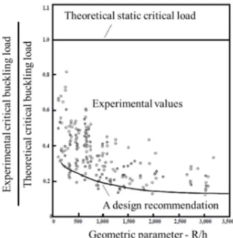
Figure 1. Comparison of the theoretical critical load of a cylindrical shell under axial load with the scatter of experimental results.
Paper received 17 April 2012. Paper accepted 3 September 2012.
Also, a considerable effort in structural engineering has been directed towards understanding the behavior of structures liable to buckling (Bazant and Cedolin, 1991). This step is essential for the development of safe design criteria (Ziemian, 2010). While a good correlation between the experimental results and the theoretical critical loads can be observed for structural elements exhibiting stable post-buckling behavior, such as plates and columns, a persistent discrepancy between theoretical and experimental buckling loads is observed for structural systems exhibiting unstable post-buckling behavior, being the experimental results lower than the theoretical ones. Figure 1 compares the normalized theoretical critical load of a perfect cylindrical shell under axial load with the scatter of experimental results found in the literature (Batista and Gonçalves, 1994). Here (R/h) is the radius-to-thickness ratio, which is a measure of the shell slenderness. The experimental results are much lower than the theoretical critical load, being the theoretical value a distant upper bound. This is an archetypal example of an imperfection sensitive structure in structural stability.
further analyzed by several authors and nowadays it is agreed that the safety of a nonlinear mechanical system or structure depends not only on the stability of their solutions, but also on the continuous and uncorrupted basin surrounding each solution, the total erosion of a given basin corresponding to the system failure. The integrity of a basin of attraction depends on the topology of the basin boundary, which can be smooth or fractal, and on the way that the basins of the various co-existing solutions interfere with each other. This topic is particularly important in systems exhibiting multiple potential well, where the basins of various in-well and cross-well solutions are intertwined. In a recent work Rega and Lenci (2005) summarized the current knowledge in the area and introduced new concepts which can be efficiently used for the integrity analysis of nonlinear systems. Recently, using these concepts, Gonçalves et al. (2011) studied the global dynamics and topological integrity of the basins of attraction of a parametrically excited cylindrical shell through a two-degree-of-freedom reduced order model. However the investigation of the influence of uncertainties and random noise on the evolution and stratification of the basins of attraction must also be carried out to arrive at a safe load level for design.
To take indirectly into account these deleterious effects, several lower bounds of static buckling loads have been proposed for design. They are usually based on the scatter of experimental buckling loads and energy considerations (Batista and Gonçalves, 1994). Estimate of the dynamic buckling load of structures with unstable post-buckling behavior – the load corresponding to escape from the safe pre-buckling well – considering the effects of uncertainties and imperfections is a much more difficult task. Structures under dynamic loads may exhibit both local and global bifurcations that affect in different ways the load carrying capacity and degree of safety of the structure. Global bifurcations are particularly important since they control, as shown by Soliman and Thompson (1989), the evolution of the basins of attraction of the solutions in phase space. In addition, compared with the static case, the number of load control parameters is higher. Finally, experimental results of dynamic buckling loads of slender structures are rather scarce in literature (Virgin, 2000; Amabili, 2008). Therefore, little is known on the effects of uncertainties on the load carrying capacity of structures liable to unstable static buckling in a dynamic environment. In a recent work Gonçalves and Santee (2008) analyzed the influence of uncertainties on the load carrying capacity of a simplified structural model exhibiting unstable post-buckling behavior. Using several tools of non-linear dynamics, they showed that the uncertainties have an influence similar and of the same order as geometric imperfections on the scatter of buckling loads and proposed a safe lower bound based on Melnikov’s criterion. Thus, the aim of the present work is, using a similar methodology, to study the influence of uncertainties on the dynamic stability of a cylindrical shell under axial loads.
The influence of combined random material and geometric properties on the free vibration frequencies and buckling loads of cylindrical shells has been investigated by, among others, Yadav and Verma (2001); Singh, Yadav and Iyengar (2002); Stefanou and Papadrakakis (2004); Papadopaulos and Papadrakakis (2005); Kriegesmann et al. (2010) and Stefanou (2011). On the other hand, there is a lack of information on the influence of these uncertainties on the post-buckling behavior and particularly on the nonlinear oscillations of these structures. However, for other systems, a number of publications, in recent years, have investigated the influence of random noise on their bifurcations, basins of attraction and the competition between different attractors (Lai and Winslow, 1994; Kraut, Feudel, and Grebogi, 1999; Kraut and Feudel, 2002). As an extension of these previous works, and following the methodology described in Gonçalves, Silva and Del Prado (2008) for the derivation of consistent reduced order models for the
nonlinear vibrations of cylindrical shells, the present work investigates the influence of small uncertainties in the physical and geometrical parameters of the shell and the unavoidable noise present in the axial excitation on the dynamic buckling loads and bifurcation diagrams. For this, a detailed parametric analysis is carried out to clarify the influence of uncertainties in load and system parameters.
Nomenclature
D = flexural stiffness of the shell, N.m E = Young’s modulus, Pa
G(P1, ω, t) = random disturbance in axial load, N/m h = thickness, m
L = length, m
m, n = number of longitudinal half-waves and circumferential waves, respectively Mx, Mθ, Mxθ = moments resultants in, respectively, axial,
circumferential and in-plane direction, N.m/m Nx, Nθ, Nxθ = force resultants in, respectively, axial,
circumferential and in-plane direction, N/m P0 = axial static pre-load, N/m
P1 = amplitude of the deterministic harmonic axial load, N/m
Pcr = classical axial buckling load, N/m
Q = parameter which expresses the quality of the fabrication process
R = radius, m t = time, s
u, v, w = axial, circumferential and transversal displacements of shell’s middle surface, m x = axial coordinate, m
W = non-dimensional parameter for transversal displacements
z = transversal coordinate, m
Greek Symbols
α = system parameter (E, υ, ρ, L, R or h)
α0 = mean value of the chosen parameter (design value) δ = standard deviation parameter
ε = non-dimensional parameter for axial coordinate Γ0 = non-dimensional parameter for axial static pre-load Γ1 = non-dimensional parameter for amplitude of the
deterministic harmonic axial load η1, η2 = linear viscous and viscoelastic material
damping coefficient υ = Poisson’s coefficient
θ = circumferential coordinate, rad ρ = mass density, kg/m³
x
σ ,σθ = stresses at an arbitrary point of shell in, respectively, axial and circumferential direction
2
GG
σ = variance of the random force amplitude
θ
τx = tangential resultant stresses at an arbitrary
point of shell
τ = non-dimensional parameter for time ω = deterministic excitation frequency, rad/s ω0 = lowest vibration frequency of the shell for
nominal values of physical and geometrical parameters, rad/s
ωl = frequency bandwidth of the excitation frequency, rad/s
Problem Formulation
Shell equation
Consider a cylindrical shell of radius R, thickness h and length
L, made of a linear elastic material with Young’s modulus E,
Poisson coefficient υ and mass density ρ. For an isotropic shell the stresses at an arbitrary point are given in terms of the middle surface strains and changes of curvature, according to Donnell’s shallow shell theory, by:
(
)
(
)
− + + − + − + − − = θ θ θ θθ θ θ θ υ υ υ υ τ σ σ x x x xx x x x x w R z w w u R v w R z w v R w z w u E , , , , , , 2 , , 2 , , 2 2 1 1 2 1 2 ) 1 ( 0 0 0 1 0 1 ) 1 ( (1)The shell is subjected to a harmonic axial load of the form:
(
P t)
G t P PP= 0+ 1cos(ω )+ 1,ω,
(2)
where P0 is the axial static pre-load, P1 is the amplitude of the
deterministic harmonic load, ω is the deterministic excitation frequency, t is time and G(P1, ω, t) is the random disturbance that
depends on the deterministic parameters P1 and ω.
The nonlinear equations of motion, considering only the transversal inertia and damping forces, are given in terms of the force and moments resultants as:
0
,
, + =
R N Nxx xθθ
(3) 0 , , + = R N Nx x
θ θ θ (4)
(
)
0 2 1 2 1 2 , , , , , 2 4 2 0 1 = + − + − + + + − ∇ + + θ θ θθ θ θ θ θθ θ η ω ρ η ρ x x x xx x x x w N R w N P N R M R M R M R w D w h wh&& & &
(5)
where η1 and η2 are, respectively, the linear viscous damping and
the viscoelastic material damping coefficients, D = Eh3/12(1 – υ 2) is the flexural stiffness of the shell, ω0 is the lowest vibration
frequency of the shell for nominal values of physical and geometrical parameters and the force and moments’ resultants are obtained by the integration of the stress components along the shell thickness as follows:
[
]
[
]
[
]
∫
[
]
∫
− − = = 2 2 2 2 , , , , , , , , h h x x x x h h x x x x dz z z z M M M dz N N N θ θ θ θ θ θ θ θ τ σ σ τ σ σ (6)For a simply-supported shell, the following boundary conditions must be satisfied:
( ) ( )
0,θ =v L,θ =0v
(7)
( ) ( )
0,θ =wL,θ =0w (8)
( )
0,θ =M( )
L,θ =0Mx x (9)
( )
0,θ
=N( )
L,θ
=0Nx x (10)
The boundary condition, Eq. (10), is a nonlinear boundary condition when written in terms of the displacements, that is:
+ + + + − = 2 , , 2 , , 2 2 1 2 1
1 θ θ
υ w R w v R w u v h E
Nx x x
(11)
The displacement field, in this work, is also required to satisfy the following conditions:
(
L2,θ)
=0u and v
( ) (
x,0=v x,2π)
(12)
The symmetry of the axial displacement field is a consequence of the adopted modal solution for the transversal displacement field and the symmetry of the boundary conditions (Eqs. (7)-(10)). In the foregoing, the following non-dimensional parameters have been introduced:
( )
2 2 1 1 0 0 o 1 3 υ ωω ω τ ε − = = Γ = Γ = Ω = = = R h E P P P P P t L x h w W cr cr cr o (13)Here Pcr is the classical axial buckling load of the shell.
General solution of the shell displacement field by a perturbation procedure
The numerical model is developed by expanding the transversal displacement component w in series in the circumferential and axial variables. From previous investigations on modal solutions for the nonlinear analysis of cylindrical shells under axial loads (Gonçalves and Batista, 1988; Gonçalves and Del Prado, 2002, 2005), it is observed that, in order to obtain a consistent modeling with a limited number of modes, the sum of shape functions for the displacements must express the nonlinear coupling between the modes and describe consistently the unstable post-buckling response of the shell as well as the correct frequency-amplitude relation.
Based on a perturbation procedure, the lateral deflection w can be described as:
( ) (
)
(
) (
)
∑
∑
∑
∑
= = = = + = 4 , 2 , 0 4 , 2 , 0 5 , 3 , 1 5 , 3 , 1 cos cos ) ( sin cos ) ( l ij k j ij i m l n k m j n i W ξ π θ τ ζ ξ π θ τ ζ (14)[
]
(
)
[
]
(
)
(
)
[
]
(
)
(
)
− + − + + + + + = ε π ε π θ τ ζ τ ζ ε π θ τ ζ θ τ ζ ε π θ τ ζ θ τ ζ m m n m n n m n n W 4 cos 4 1 2 cos 4 3 2 cos ) ( ) ( 3 sin ) 3 ( cos ) ( ) ( cos ) ( sin ) 3 ( cos ) ( ) ( cos ) ( 22 02 33 13 31 11 (15)The in-plane displacements u and v are obtained by substituting Eq. (15) into the in-plane equilibrium equations, Eq. (3) and Eq. (4), and by solving the system of linear partial differential equations in u and v and imposing the relevant boundary, symmetry and continuity conditions. Based on this procedure one obtains the necessary number of in-plane modes and writes their modal amplitudes in terms of the modal amplitudes ζij(t) in Eq. (15) (Gonçalves, Silva
and Del Prado, 2008; Silva, Gonçalves and Del Prado, 2011). Finally, by substituting the adopted expansion for the transversal displacement w together with the obtained expressions for u and v into the equation of motion in the transversal direction, Eq. (5), and by applying the standard Galerkin method, a consistent discretized system of ordinary differential equations of motion is derived.
Simulation of the uncertainties in the physical and geometric parameters
The physical parameters (E, υ and ρ) and the geometrical parameters (L, R and h) of the shell usually have some reference values which are defined at the stage of design. However, depending on the allowable tolerances in the fabrication process, small variations of these parameters may occur. Usually these small variations have a negligible influence on the load capacity of the structure. But in structural systems liable to buckling, due mainly to the inherent nonlinearity of the buckling process, small changes may lead to significant changes in the load capacity and safety of the structure.
For each physical and geometrical parameter, α, the following uniform probability density function, f, is assumed (Gonçalves and Santee, 2008):
( )
+ < < − = otherwise Q Q if Q f , 0 100 100 , 2 100 0 0 0 0 0 α α α α α αα (16)
where α is the system parameter (E, υ, ρ, L, R or h), α0 is the mean
value of the chosen parameter (design value), and Q is a parameter which expresses the quality of the fabrication process as a percentage of the mean value, α0.
Simulation of the random force
For the numerical calculations of the present work, the non-deterministic term of the axial load in Eq. (2), G(P1, ω, t), is
considered as a stationary and ergodic continuous stochastic process in time (Gonçalves and Santee, 2008). Another hypothesis is that the stochastic process G(P1, ω, t) has a zero expected value, that is:
(
)
[
GP1, ,t]
=0E ω (17)
The description of a stochastic process is usually made in the frequency domain. Here, it is assumed that the random term
G(P1, ω, t) has a spectral density function given by:
l GG GG ω σ ω 2 ) ( 2 =
Φ for
2 2
l
l ω ω
ω < <Ω+
− Ω
(18)
where
σ
GG2 is the variance of the random force amplitude and ωl is the frequency bandwidth of the excitation frequency.Additionally, it is considered that the standard deviation of the random force amplitude is proportional to the deterministic force amplitude, P1, thus:
1
P GG δ
σ =
(19)
where δ is the standard deviation parameter of proportionality. So, the random force is a stochastic process that depends on the frequency, ω, and amplitude, P1, of the deterministic term. The
numerical algorithms used in the present work can be found in Gonçalves and Santee (2008).
Numerical Results
Consider a cylindrical shell of radius R = 0.2 m, length L = 0.4 m and thickness h = 0.002 m. The shell material has the following properties: E = 210 GPa, υ = 0.3 and ρ = 7850 kg/m³. For this shell geometry the lowest buckling load as well as the lowest natural frequency are obtained for m = 1 and n = 5 (Gonçalves and Del Prado, 2005). The viscous and material damping coefficients, η1 and η2, are, respectively, 0.0008 and 0.0001. These values will be used throughout the present numerical analysis. These values are based on the experimental results by Amabili and co-workers (Amabili, 2008).
Numerical results with physical and geometrical uncertainties
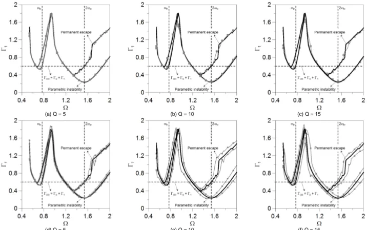
The continuous black curves in Figs. 2 and 3 are the parametric and permanent escape boundaries in the force control space, considering a deterministic harmonic axial load in Eq. (2) (G(P1, ω, t) = 0). The dashed horizontal line represents the critical
static axial load, Γcr = Γ0 + Γ1. The dashed vertical lines identify the
lowest natural frequency of the shell and twice this value, which corresponds to the main parametric resonance region. The region below the parametric instability boundary corresponds to sets of load parameters (frequency/forcing amplitude) that lead to stable trivial solutions, that is, under small perturbations the perturbed response tends to zero as time increases. The region above the escape boundary corresponds to force parameters that lead to escape from the pre-buckling well. After escape, the shell may exhibit small amplitude oscillations around a post-buckling equilibrium position or large cross-well motions. Between these two regions, there is a region with a complex dynamics where, depending on the initial conditions, the shell may display harmonic or sub-harmonic motions within the buckling well or escape from the pre-buckling well. In this region, the dynamic response and, consequently, the dynamic buckling load are rather sensitive to physical and geometrical uncertainties.
(a) Q = 5 (b) Q = 10 (c) Q = 15
(d) Q = 5 (e) Q = 10 (f) Q = 15
Figure 2. Parametric and escape instability boundaries in the force control space, considering an uncertainty in the Young modulus, E. (ΓΓΓΓ0 = 0.40,
G(P1, ωωωω, t) = 0).
(a) Q = 5 (b) Q = 10 (c) Q = 15
(d) Q = 5 (e) Q = 10 (f) Q = 15
Figure 3. Parametric and escape instability boundaries in the force control space, considering an uncertainty in the shell thickness, h. (ΓΓΓΓ0 = 0.40,
The curves in gray in Figs. 2a-c and 3a-c represent, respectively, the mean parametric instability boundary and escape boundary, obtained using the arithmetic mean value of the ten critical loads. The curves in gray in Figs. 2d-f and 3d-f illustrate, respectively, the parametric and escape instability boundaries considering the average value plus or minus the standard deviation of ten samples.
The stability boundaries shown in Figs. 2a-c and 3a-c obtained by the mean value of the critical loads are slightly different from those obtained for the reference system. This difference increases with the value of Q. In all cases the upper and lower bounds of the ten samples, as shown in Figs. 2f and 3f, lead to a high variability of the critical loads, especially on the right hand side of the main parametric instability region where the parametric instability is characterized by a super-critical bifurcation leading to a period two solution. The critical load is particularly sensitive to the small variations in the shell thickness, as expected for a thin-walled structure.
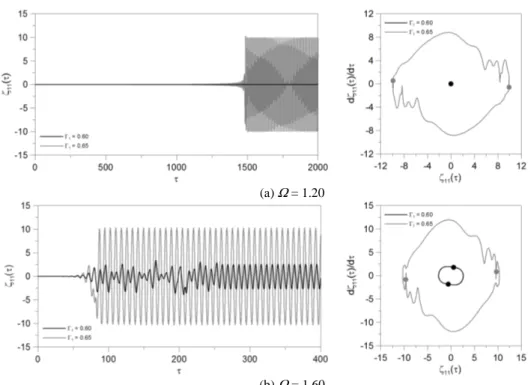
Figure 4 illustrates the possible types of the shell response in the vicinity of each stability boundary shown in Fig. 2 through time responses, projections of the phase space and Poincaré sections (dots along the phase space projections). If the cylinder is subjected to a periodic axial load, it will undergo the familiar longitudinal forced vibration, exhibiting a uniform transversal motion, due to the effect of
Poisson’s ration, also known as breathing mode. However at certain critical values, the longitudinal motion becomes unstable and the cylinder executes transverse bending vibrations. In Fig. 4a, for a forcing amplitude lower than the critical value (Γ1 = 0.60) and Ω = 1.20, after a small initial disturbance, the amplitude of the response decreases rapidly converging to the trivial solution. If the control parameter Γ1 is increased slightly beyond the critical value, (Γ1 = 0.65), the shell exhibits initially an exponential growth of the amplitude, as predicted by the linear theory, converging to a limit cycle within the pre-buckling well. In this case the trivial solution becomes unstable and the system converges to a period-two stable solution (a period-k response means a steady state response with a period k times that of the forcing). Figure 4b illustrates the shell response in the vicinity of the escape boundary. For Γ1 = 0.60 and Ω = 1.60 the response converges to a limit cycle of period two within the pre-buckling well. For Γ1 = 0.65 the motion can no longer remain within the pre-buckling well and converges to a remote attractor, exhibiting large amplitude cross-well motions. These possible outcomes are rather sensitive to initial conditions and system parameters. So, small variations on these data may lead to different system responses, which may affect the safety of the structure.
(a) Ω = 1.20
(b) Ω = 1.60
Figure 4. Time responses, phase-portraits and Poincaré maps. (ΓΓΓΓ0 = 0.40, G(P1, ωωωω, t) = 0). Sample 3 (E = 224,87 GPa) – Q = 10.
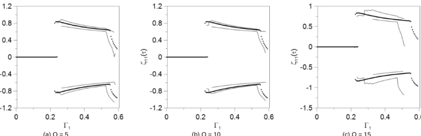
Figures 5-8 show characteristic bifurcation diagrams of the left and right hand sides of the main parametric instability region. Figures 5 and 7 correspond to sub-critical bifurcations representative of the left hand side of the instability region while Figs. 6 and 8 correspond to super-critical bifurcation representative of the right hand side of the instability region. These bifurcation diagrams are obtained by the brute force method which maps a sequence of stable responses as the bifurcation parameter increases. They are obtained by fixing the forcing frequency and increasing slowly the forcing amplitude.
The black curves are the coordinate ζ11(τ) of the Poincaré map
of the reference solution obtained with the design values. The gray
curves represent the lower and upper bounds of the coordinate ζ11(τ)
of the Poincaré map considering the ten different samples. Figures 5 and 6 show the influence of the uncertainties in the value of the Young modulus while Figs. 7 and 8 illustrate the influence of small variations in the shell thickness.
(a) Q = 5 (b) Q = 10 (c) Q = 15
Figure 5. Bifurcation diagram considering an uncertainty in the Young modulus. ΓΓΓΓ0 = 0.40, ΩΩΩΩ = 1.50, G(P1, ωωωω, t) = 0.
(a) Q = 5 (b) Q = 10 (c) Q = 15
Figure 6. Bifurcation diagram considering an uncertainty in the Young modulus. ΓΓΓΓ0 = 0.40, ΩΩΩΩ = 1.80, G(P1, ωωωω, t) = 0.
(a) Q = 5 (b) Q = 10 (c) Q = 15
Figure 7. Bifurcation diagram considering an uncertainty in the shell thickness. ΓΓΓΓ0 = 0.40, ΩΩΩΩ = 1.50, G(P1, ωωωω, t) = 0.
(a) Q = 5 (b) Q = 10 (c) Q = 15
(a) sample 3 (E = 224,87 GPa) – Q = 10
(b) sample 5 (E = 237,05 GPa) – Q = 10
Figure 9. Two samples of the bifurcation diagram considering an uncertainty in Young modulus. ΓΓΓΓ0 = 0.40, ΩΩΩΩ = 1.80, G(P1, ωωωω, t) = 0.
Figure 10. Phase-portrait and Poincaré map for ΓΓΓΓ0 = 0.40, ΓΓΓΓ1 = 1.00, ΩΩΩΩ =
1.80, G(P1, ωωωω, t) = 0. Uncertainty in Young modulus.
Figure 10 shows two different shell responses when an uncertainty in Young modulus is considered. While in one case a period two response is observed, in the other the steady state response exhibit a period four times greater than that of the forcing. While the former results from one period doubling bifurcation, the latter is the result of two period doubling bifurcations. This shows that small variations in one parameter may lead to different bifurcation scenarios.
Numerical results with random forces
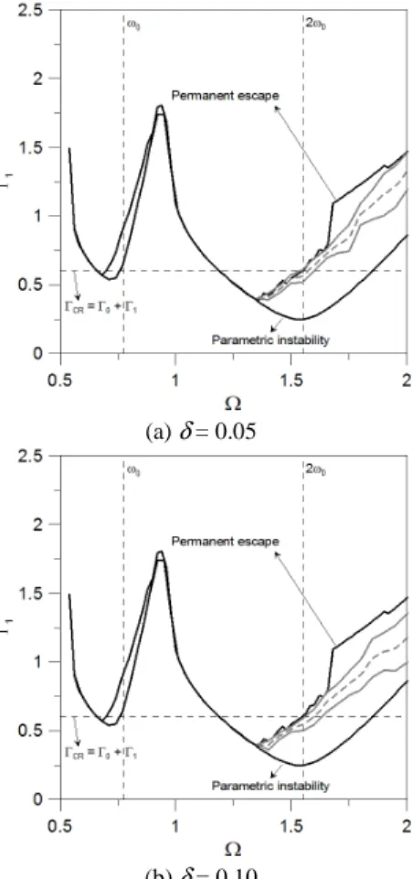
Figure 11 shows the influence of the random portion of the load,
G(P1, ω, t), described by Eq. (2), on the parametric instability and
escape boundaries of the axially loaded cylindrical shell for one bandwidth, ωl, 0.50 and two values of the standard deviation parameter, δ, 0.05 and 0.10. For this value of ωl and δ ten samples are generated and the two critical loads are evaluated, considering the average values of the shell geometry and physical parameters. In Fig. 11, curves in black are the results for a deterministic harmonic force, as shown in Figs. 2 and 3. The dashed gray curves represent the average of the escape load. The presence of noise leads to a dispersion of the results in the right side of the instability region. The continuous gray curves represent the value of the mean load added or subtracted from the value of the standard deviation of ten samples. As the standard deviation parameter, δ, increases, the dispersion of the dynamic buckling loads increase. Also all escape loads of the perturbed system are lower than the permanent escape load of the shell under a deterministic load. So, the shell is sensitive to noise in the excitation and this decreases the safety of the shell in a dynamic environment.
(a) δ = 0.05
(b) δ = 0.10
Figure 11. Instability boundaries in force control space. (ΓΓΓΓ0 = 0.40,
ω ωω ωl = 0.50).
Figure 12 shows two time responses considering the same set of force parameters (Γ0 = 0.40, Γ1 = 0.675, Ω = 1.60, ωl = 0.25,
deterministic load displays a sub-harmonic response of period two, the perturbed system exhibit a quasi-periodic motion.
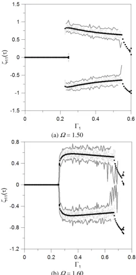
Figure 13 illustrates the characteristic bifurcation diagrams of the main parametric instability region considering Γ0 = 0.40,
ωl = 0.25, δ = 0.10. Figure 13a shows a sub-critical bifurcation representative of the shell behavior on the left hand side of the main instability region, while Fig. 13b illustrates the behavior of the shell on the right hand side of the main instability region. The black dots represent the coordinate ζ11(τ) of the Poincaré map of the shell
under deterministic harmonic load, while the two gray curves represent the bounds of the coordinates of the Poincaré map obtained after ten samples of the perturbed load (gray dots). The results show that the random small perturbation of the harmonic forcing does not change the overall behavior and bifurcations of the system, causing only small perturbations of the Poincaré map around the fixed points of the deterministic system due to the perturbations of the orbit as illustrated in Fig. 13. The dispersion of points around the fixed points increases as δ increases.
Figure 12. Time response and phase portrait of the cylindrical shell under random noise. (ΓΓΓΓ0 = 0.40, ΓΓΓΓ1 = 0.675, ΩΩΩΩ = 1.60, ωωωωl = 0.25, δδδδ = 0.10).
(a) Ω = 1.50
(b) Ω = 1.60
Figure 13. Bifurcation diagrams of the cylindrical shell. (ΓΓΓΓ0 = 0.40,
ω ωω
ωl = 0.25, δδδδ = 0.10).
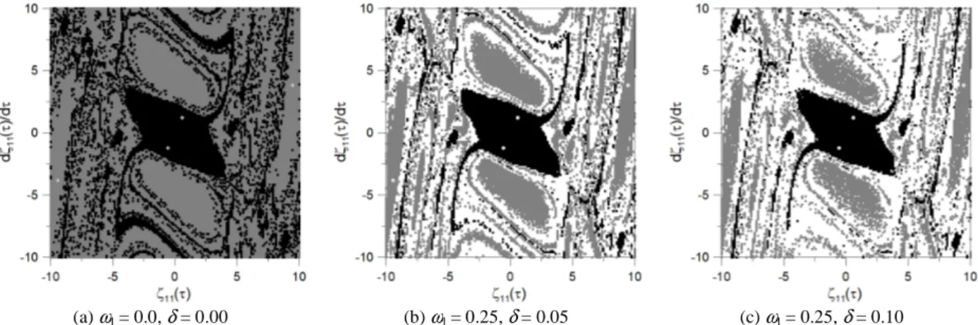
Figure 14 illustrates the influence of random noise on the basin of attraction of the shell considering Γ0 = 0.40, Γ1 = 0.40, Ω = 1.60. It shows three cross-sections of the twelve-dimensional basin of attraction by the ζ11(τ) x dζ11(τ)/dτ plane. A total of 150 x 150 cells
are considered in the analysis. The black region corresponds to the initial conditions that converge to the period two attractor within the pre-buckling well, while the gray region corresponds to initial conditions that lead to a period two large-amplitude solution outside the pre-buckling well. Figure 14a corresponds to the deterministic case and Fig. 14b and Fig. 14c are related to perturbed solutions obtained with δ = 0.05 and δ = 0.10, respectively, and ωl = 0.25. In the deterministic case each set of initial conditions leads to a specific attractor. In the non-deterministic case, for each set of initial conditions, the equations of motion are integrated using ten different samples of random perturbation. If in all cases all responses converge to the same attractor as in the deterministic case, the cell is either marked in black or gray, but if they converge to different attractors or if the attractor is different from the one identified in the deterministic case, this means that the response associated with a given set of initial conditions is sensitive to random noise and the cell is marked in white in Fig. 14b and Fig. 14c. As the standard deviation parameter δ increases the white region increases, decreasing the safe region associated with a given attractor.
Figure 15 shows the probability density function of the initial conditions used for the construction of the basins of attraction of Fig. 14. In these figures 22500 sets of initial conditions randomly distributed in the plane ζ11(τ) x dζ11(τ)/dτ are used and, for each set,
(a) ωl = 0.0, δ = 0.00 (b) ωl = 0.25, δ = 0.05 (c) ωl = 0.25, δ = 0.10
Figure 14. Cross sections of the basin of the attraction of the shell submitted to (a) a deterministic and (b, c) non-deterministic load. (ΓΓΓΓ0 = 0.40, ΓΓΓΓ1 = 0.40,
Ω Ω Ω Ω = 1.60).
(a) ωl = 0.0, δ = 0.00 (b) ωl = 0.25, δ = 0.05
(c) ωl = 0.25, δ = 0.10
Figure 15. Probability density functions for the set of initial conditions analyzed in Fig. 14. (ΓΓΓΓ0 = 0.40, ΓΓΓΓ1 = 0.40, ΩΩΩΩ = 1.60). Conclusions
In this work Donnell’s shallow shell equations are used to study the nonlinear vibrations and instabilities of a simply-supported cylindrical shell. A reduced order model is derived, which satisfies the relevant boundary, continuity and symmetry conditions of the problem and describes with precision the shell motions up to large deflections. The parametric analysis clarifies the influence of small uncertainties of physical parameters and geometry of the shell on the parametric instability and escape
bifurcation connected with the observed instability phenomena, namely, parametric instability and escape from the pre-buckling well. However, in a slowly evolving system the random noise may decrease the escape load in certain excitation frequency ranges. Also, it adds a certain degree of uncertainty to the basin boundaries decreasing the safe region of the shell. The results show that in structures liable do instability, the effect of small uncertainties must be taken into account in the definition of reliable safety factors for design.
Acknowledgements
The authors acknowledge the financial support of the Brazilian research agencies CAPES, CNPq and FAPERJ.
References
Amabili, M., 2008, “Nonlinear Vibrations and Stability of Shells and Plates”, Cambridge University Press, Cambridge, United Kingdom, 374 p.
Amabili, M. and Païdoussis, M.P., 2003, “Review of studies on geometrically nonlinear vibrations and dynamics of circular cylindrical shells and panels, with and without fluid-structure interaction”, Applied Mechanics Reviews, Vol. 56, pp. 655-699.
Batista, R.C. and Gonçalves, P.B., 1994, “Non-Linear Lower Bounds for Shell Buckling Design”, Journal of Constructional Steel Research, Vol. 29, pp. 101-120.
Bazant, Z. and Cedolin, L., 1991, “Stability of Structures”, Oxford University Press, Oxford, United Kingdom, 1011 p.
Chu, H.N., 1961, “Influence of large amplitudes on flexural vibrations of a thin circular cylindrical shells”, Journal of Aerospace Science, Vol. 28, pp. 302-609.
Evensen, D.A., 1963, “Some observations on the nonlinear vibration of thin cylindrical shells”, AIAA Journal, Vol. 1, pp. 2857-2858.
Evensen, D.A., 1967, “Nonlinear flexural vibrations of thin-walled circular cylinders”, NASA TN, D-4090.
Gonçalves, P.B. and Batista, R.C., 1988, “Nonlinear vibration analysis of fluid-filled cylindrical shells”, Journal of Sound and Vibration, Vol. 127, pp. 133-143.
Gonçalves, P.B. and Del Prado, Z.J.G.N., 2002, “Nonlinear oscilations and stability of parametrically excited cylindrical shells”, Meccanica, Vol. 37, pp. 569-597.
Gonçalves, P.B. and Del Prado, Z.J.G.N., 2005, “Low-dimensional Galerkin model for nonlinear vibration and instability analysis of cylindrical shells”, Nonlinear Dynamics, Vol. 41, pp. 129-145.
Gonçalves, P.B. and Santee, D.M., 2008, “Influence of Uncertainties on the Dynamic Buckling Loads of Structures Liable to Asymmetric Post-Buckling Behavior”, Mathematical Problems in Engineering, Vol. 2008, pp. 1-24.
Gonçalves, P.B., Silva, F.M.A., and Del Prado, Z.J.G.N., 2008, “Low-dimensional models for the nonlinear vibration analysis of cylindrical shells based on a perturbation procedure and proper orthogonal decomposition”, Journal of Sound and Vibration, Vol. 315, pp. 641-663.
Gonçalves, P.B., Silva, F.M.A., Rega, G. and Lenci, S., 2011, “Global dynamics and integrity of a two-dof model of a parametrically excited cylindrical shell”, Nonlinear Dynamics, Vol. 63, pp. 61-82.
Koiter, W.T., 1945, “On the stability of elastic equilibrium”, PhD dissertation, Delft, Holland.
Kounandis, A.N., 2006, “Recent advances on postbuckling analyses of thin-walled structures: Beams, frames and cylindrical shells”, Journal of Constructional Steel Research, Vol. 62, pp. 1101-1115.
Kraut, S., and Feudel, U., 2002, “Multistability, noise, and attractor hopping: The crucial role of chaotic saddles”, Physical Review E – Rapid Communications, Vol. 66, pp. 1-4.
Kraut, S., Feudel, U., and Grebogi, C., 1999, “Preference of attractors in noisy multistable systems”, Physical Review E, Vol. 59, pp. 5253-5260.
Kriegesmann, B., Rolfes, R., Hühne, C., Teβmer, J., and Arbocz, J., 2010, “Probabilistic design of axially compressed composite cylinders with geometric and loading imperfections”, International Journal of Structural Stability and Dynamics, Vol. 10, pp. 623-644.
Lai, Y-C., and Winslow, R.L., 1994, “Fractal basin boundaries in coupled map lattices”, Physical Review E, Vol. 50, pp. 3470-3473.
Nowinski, J.L., 1963, “Nonlinear transverse vibration of orthotropic cylindrical shells”, AIAA Journal, Vol. 1, pp. 617-620.
Olson, M.D., 1965, “Some experimental observations on the nonlinear vibrations of cylindrical shells”, AIAA Journal, Vol. 3, pp. 1775-1777.
Papadopoulos, V. and Papadrakakis, M., 2005, “The effect of material and thickness variability on the buckling load of shells with random initial imperfections”, Computer Methods in Applied Mechanics and Engineering, Vol. 194, pp. 1405-1426.
Rega, G. and Lenci, S., 2005, “Identifying, evaluating and controlling dynamical integrity measures in non-linear mechanical oscillators”, Nonlinear Analysis, Vol. 63, pp. 902-914.
Santee, D.M., 1999, “Non-linear vibrations and instabilities of imperfection-sensitive structural elements”, D. Sc. Thesis, Civil Engineering Department, Catholic University, PUC-Rio, Rio de Janeiro, Brazil, 250 p.
Silva, F.M.A., Gonçalves, P.B., and Del prado, Z.J.G.N., 2011, “An alternative procedure for the non-linear vibration analysis of fluid-filled cylindrical shells”, Nonlinear Dynamics, Vol. 66, pp. 303-333.
Singh, B.N, Yadav, D. and Iyengar, N.G.R., 2002, “Free vibration of compostie cylindrical panels with random material properties”, Composite Structures, Vol. 58, pp. 435-442.
Soliman, M.S. and Thompson, J.M.T., 1989, “Integrity measures quantifying the erosion of smooth and fractal basins of attraction”, Journal of Sound and Vibration, Vol. 135, pp. 453-475.
Soliman, M.S. and Thompson, J.M.T., 1992, “Global Dynamics Underlying Sharp Basin Erosion in Nonlinear Driven Oscillators”, Physical Review A, Vol. 45, pp. 3425-3431
Stefanou, G., 2011, “Response variability of cylindrical shells with sthocastic non-Gaussian material and geometric properties”, Engineering Structures, Vol. 33, pp. 2621-2627.
Stefanou, G., and Papadrakakis, M., 2004, “Sthocastic finite element analysis of shells with combined random material and geometric properties”, Computer Methods in Applied Mechanics and Engineering, Vol. 193, pp. 139-160.
Thompson, J.M.T., 1989, “Chaotic behavior triggering the escape from a potential well,” Proceedings of Royal Society London A, Vol. 421, pp. 195-225. Virgin, L.N., 2000, “Introduction to Experimental Nonlinear Dynamics”, Cambridge University Press, Cambridge, United Kingdom, 256 p.
Yadav, D. and Verma, N., 2001, “Free vibration of composite circular cylindrical shells with random material properties. Part II: Applications”, Composite Structures, Vol. 51, pp. 371-380.