Douglas D. Bueno
[email protected]Clayton R. Marqui
[email protected]Luiz C. S. G ´oes
[email protected] Technological Institute of Aeronautics S˜ao Jos´e dos Campos 12228-900 SP – BrazilPaulo J. P. Gonc¸alvez
[email protected] Universidade Estadual Paulista Bauru 17033-360 SP – BrazilAeroelastic Stability Analysis Using
Linear Matrix Inequalities
The present work describes an alternative methodology for identification of aeroelastic stability in a range of varying parameters. Analysis is performed in time domain based on Lyapunov stability and solved by convex optimization algorithms. The theory is outlined and simulations are carried out on a benchmark system to illustrate the method. The classical methodology with the analysis of the system’s eigenvalues is presented for comparing the results and validating the approach. The aeroelastic model is represented in state space format and the unsteady aerodynamic forces are written in time domain using rational function approximation. The problem is formulated as a polytopic differential inclusion system and the conceptual idea can be used in two different applications. In the first application the method verifies the aeroelastic stability in a range of air density (or its equivalent altitude range). In the second one, the stability is verified for a range of velocities. These analyses are in contrast to the classical discrete analysis performed at fixed air density/velocity values. It is shown that this method is efficient to identify stability regions in the flight envelope and it offers promise for robust flutter identification.
Keywords:flutter analysis, LMI, Lyapunov function, time domain
Introduction
In problems of fluid and flexible structure interactions various physical phenomena can be observed and also, because of its catastrophic nature, flutter is an important topic involving aeroelastic stability. This phenomenon is an interaction between the structural dynamics and the aerodynamics that results in divergent and destructive oscillations of motion (Bisplinghoff et al., 1996).
Different approaches have been proposed to identify the flutter boundaries. In general, the methods are formulated in frequency domain as eigenvalue problems, for which the aeroelastic model is defined for each point in the flight envelope (a pair of altitude and velocity). Details can be found in Theodorsen and Garrick, 1940; Hassig, 1971; and Chen, 2000. This can be costly in terms of computational time and engineering analysis of data if a large number of points need to be calculated. Also, the uncertainties in the aircraft model makes the prediction of the stability boundary difficult (Chung et al., 2008).
In modern development, authors have introduced robust flutter analysis including structural and aerodynamics uncertainties. Initially, Lind and Brenner (1999) introduced structured singular value µ into the aeroelastic field and developed a µ-method in which the aeroelastic system is parametrized with dynamic pressure perturbations. Chung et al. (2008) included aerodynamic uncertainties by considering variation of Mach number, which is represented by the boundary of Theodorsen’s lift deficiency function. Chung and Shin (2010) defined the worst case flutter boundary by considering the structural variation due to changing natural frequency and aerodynamic variation and, according to the authors, this approach is more conservative than a nominal case.
In this context, this paper proposes an alternative approach to include uncertainties in the aeroelastic stability problems. Two applications are introduced at which the problem is formulated as a polytopic differential inclusion system considering uncertainties in the air density (or its equivalent altitude) or in the airspeed. The main idea is to identify regions of stability in the flight envelope by solving a linear matrix inequality. The method is written in time domain using the state space realization and the Theodorsen’s aerodynamic model using a by rational function approximation for the aerodynamic forces. This methodology offers promise for robust flutter analysis
Paper received 1 May 2012. Paper accepted 22 July 2012.
using convex optimization.
Nomenclature
s = Laplace variable M = mass matrix D = damping matrix K = stiffness matrix Q = aerodynamic matrix u = vector of displacement A = dynamic matrix C = output matrix x = vector of states y = vector of output b = semi chord k = reduced frequency Nlag = number of lags
v = number of vertices V = airspeed
VLyap = Lyapunov energy function
q = dynamic pressure mM = Mach number
M = airfoil mass
Greek Symbols
β = parameter of lag
δ = differential inclusion
ρ = air density Ω = convex space
ωh = airfoil oscillation plunge frequency ωθ = airfoil oscillation pitch frequency ωβ = frequency of control surface deflection
Subscripts
a = relative to aerodynamic lags m = relative to modal coordinates p = relative to physical domain unc = relative to uncertain parameter
Superscripts
Aeroelastic Model
The aeroelastic model is characterized by the mass, stiffness, damping and aerodynamic matrices. These matrices are typically obtained from finite element method and the system is commonly represented in frequency domain using modal coordinates. In this case, the equation of motion is written as
s2Mmum(s) +sDmum(s) +Kmum(s) =qQm(mM,k)um(s) (1)
where the subscriptmindicates the modal coordinates. Aerodynamic matrices can be obtained using the Doublet Lattice method in a constant Mach number(mM)for each reduced frequencyk(Albano and Rodden, 1969). However, in this work they are computed using the Theodorsen’s aerodynamic theory. The method proposed requires a representation in time domain of the system, in Eq. (1), but because the termQm(mM,k)has no Laplace inverse, it is necessary to write it in terms of rational function approximation, so that the aerodynamic forces can be transformed to time domain. This is done using Roger’s approximation (Roger, 1977), given by Eq. (2). Its contains a polynomial part representing the forces on the section acting directly connected to the displacementsu(t)and their first and second derivatives. Also, this equation has a rational part representing the influence of the wake acting on the section with a time delay.
Qm(s) =
" 2
∑
j=0
Qm jsj
b V
j
+
nlag
∑
j=1
Qm(j+2) s s+Vbβj
!#
um(s)
(2)
wheresis the Laplace variable,nlagis the number of lag terms and βjis thejth lag parameter(j=1,···,nlag).
Substituting Eq. (2) into Eq. (1), it is possible to obtain, after some rearrangements, the classical aeroelastic equation of motion in a state space format as:
˙x(t) =Ax(t) and y(t) =Cx(t) (3)
wherex(t) ={˙umumuam}T is the state vector anduamare states of lags required for the approximation. The output matrixC= [CvCd] has dimension 2m×m(2+nlag), whereCvandCd, respectively the velocity and displacement, are output vectors. MatrixAis presented in the following form:
A=
−M−am1Dam −M−am1Kam A3
A4 A5 A6
(4)
where
Mam=Mm−q
b V
2
Qm2
Dam=Dm−q
b V
Qm1=Dm−ρ0.5V bQm1
Kam=Km−qQm2=Km−ρ0.5V2Qm0
A3=
h
qMam−1Qm3 ···qMam−1Qm(2+nlag)
i
(5)
and matricesAj, for j=4,5,6, are defined in the appendix.
In classical solutions the aeroelastic stability is treated as an eigenvalue problem of the dynamic matrix A. Frequency of oscillation and damping are extracted from the complex eigenvalues. This analysis is performed for fixed values of velocity and air density (V,ρ).
In Eq. (4), matrix A has a termMam that has to be inverted. For mass normalized eigenvectors,Mm=I(identity matrix), so the inverse of the aeroelastic mass matrix can be rewritten as
M−am1=I−ρ0.5b2Qm2
−1
(6)
For the cases where −ρ0.5b2Qm2 j
vanishes whenjis large, the Taylor expansion can be used as an approximation of Eq. (6) and then, it can be written as
M−am1≈I+
NT
∑
j=1
(−1)jρj−0.5b2Qm2
j
(7)
whereNTis a positive natural number chosen conveniently.
For the problem considered in this paper, the assumption −ρ0.5b2Qm2
j
→ 0 when j→∞has shown to be true. When this assumption is not satisfied, it is possible to use another approximation for the inverse ofMam. Different methods to compute the inverse of sum of matrices can be found in Petersen and Pedersen, 2008, and Henderson and Searle, 1981.
When this assumption is satisfied, the approximated state space matrix of Eq. (3) can be written as
Aapp=
A1 A2 A3
A4 A5 A6
(8)
where the submatricesA1,A2, ...,A6are given in the appendix.
Continuous Range Stability Analysis
The objective of a continuous stability analysis is to introduce a robust procedure for checking if flutter is present in a range of a varying parameter. In the classical method, the discrete analysis is performed by reducing the intervals of a varying parameter, such as velocity or air density, which can be costly for analysis of a full flight envelope. Two procedures are presented here, the first considers a fixed velocity and analysis is carried out for a range of air density. The second procedure is formulated for fixed value of air density and varying parameter is now velocity.
Procedure 1: Analysis for air density range
Considering the aeroelastic model written in state space format to describe a range of altitude for a fixed value of velocity, as illustrated in Fig. 1. A convex space is obtained using a polytopic differential inclusion system (PLDI) and the air density given by
ρunc=ρ+∆ρ=ρ(1+δ) (9)
where the subscriptunc indicates the uncertain air densityρ andδ
denotes its associated uncertainty. In this case, the aeroelastic model is written as a PLDI system and the dynamic matrix is given by
A=A(ρunc,ρ2unc,···,ρ j
unc,···,ρNuncT+1) (10)
and, ifρuncj =ρj(1+δj), then
A=A(δ1,···,δ(NT+1)) =Aunc (11)
Airspeed
A
lt
it
u
d
e
∆ρ1
Vj
∆ρ2 ∆ρj
∆ρnρ
Vmax
Figure 1. Procedure 1 - Air-Density Robust Analysis.
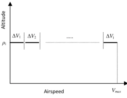
Procedure 2: Analysis for a velocity range
Considering the system of Eq. (3) to be written in state space format as a PLDI system and its convex space representing an airspeed range as shown in Fig. 2, the uncertainty range can be written as
Vunc=V+∆V=V(1+δv) (12)
where the subscriptunc indicates the uncertain airspeedV and δv denotes its associated range in terms of percentage. In this case, the aeroelastic model is written as a PLDI system and the dynamic matrix is given by
A=A(Vunc,Vunc2 ) (13)
and, ifVunc2 =V2(1+δ2v), then
A=A(δ1v,δv2) =Aunc (14)
whereδv1andδ2vare understood as uncertain parameters related to that polytopic system and physically they represent the airspeed range. In this case the maximum and minimum values ofδvj(j=1,2)are given by
δv j=
V+∆V V
j
−1 (15)
SubstitutingVbyVunc=V(1+δv1)andV2byVunc2 =V2(1+δ2v)
into Eq. (4) it is possible to define the dynamic matrix that describes the PLDI system and represents the velocity range[V,V+∆V]. In this case, the convex space is geometrically represented by a plane.
Lyapunov Energy Function
Consider the energy functionVLyap(t) =xTPx. The aeroelastic system defined in a particular pair air density and velocity is stable if
d
dt[VLyap]<0 (16)
Equation (16) represents the energy dissipation over time, idea which has been proposed by Alexander Lyapunov (in 1907). The
Airspeed
A
lt
it
u
d
e
∆V1 ∆V2 ∆Vj
ρi
…..
Vmax
Figure 2. Procedure 2 - Robust velocity analysis
method is traditionally applied to the stability analysis in control theory because Lyapunov showed that the differential equation (Eq. (3)) is stable if and only if exists a positive-definedPsuch that (Boyd et al., 1994)
˙
VLyap(t) =˙xTPx+xTP˙x=xTATuncPx+xTPAuncxT
˙
VLyap(t) =xT ATuncP+PAuncx, or
ATuncP+PAunc<0
(17)
Equation (17) is called Lyapunov inequality on P and its first application in practical control engineering problems was introduced in the early 1960’s (Boyd et al., 1994).
Quadratic stability criteria for aeroelastic analysis
Consider a PLDI system given by
˙x(t) =Auncx(t) =A(α)x(t) (18)
where the dynamic matrixA(α) belongs to a convex polytopic set defined as
Co:=
(
A(α):A(α) =
v
∑
j=1 αrjArj
)
(19)
where∑vj=1αrj=1 andαrj≥0,∀j=1,···,v(Oliveira et al., 1999).
Also, v is the number of vertices of the polytopic system and rj denotes its jth vertex. The number of vertices is given by 2(NT+1)
for application 1 (and 22=4 for application 2) and the operatorCo
means that matricesAr1,···,Arv define the desired convex spaceΩ
(Boyd et al., 1994).
Substituting Eq. (19) into inequality (17), the Lyapunov inequality is rewritten as
rv
∑
j=1 αrjArj
!T
P+P
rv
∑
j=1 αrjArj
!
<0 (20)
Pre and post multiplying the last LMI byX=P−1and after some rearrangement, the quadratic stability criteria is written as
αr1
Ar1X+XA
T r1
+···+αrv
ArvX+XA
T rv
The necessary condition to ensure the quadratic stability of the aeroelastic system into this convex space is to solve Eq. (21) at its vertices for whichA(α) =Arj withαrj=1 andαk=0,∀k6= j. In
this case, all LMIs must be satisfied simultaneously (Barmish, 1985).
Ar1X+XA
T r1<0
.. . ArjX+XA
T rj<0
.. . ArvX+XA
T rv<0
(22)
The vertices of the parameter box (or the convex space) are a combination of the minimum and maximum values of the parameters of the system. It is supposed that the system can assume any combination of values inside the box (Boyd et al., 1994; Silva and Lopes Jr., 2006).
Lyapunov Stability Index
In order to identify regions into the flight envelope at which system is stable, the Lyapunov stability index is defined to classify the regions of aeroelastic stabilities. Particular details are presented here and the conceptual understanding is the same for both applications.
Application 1: Robust air-density analysis
The convex spaceΩ∈R(NT+1)must be understood as a fictitious
domain at which the aeroelastic stability is verified. The main reason is that although the product(ρδ1)∈R∗+represents a physical parameter variation, the parameters (ρjδj), j=2,···,NT+1, are introduced only for creating the convex space and they have no physical information. However, the physical domainΩp ⊂Ωand then:
• if there isXsuch that all inequalities in (22) are simultaneously feasible⇒the system is stable inΩand stable inΩp. So,
σLyap=1 (23)
• otherwise⇒the system is not stable inΩ. So,
σLyap=−1 (24)
whereΩp:=(ρ,ρ+∆ρ) and Vj | Ωp ∈R. If the proposed Lyapunov stability index isσLyap=−1, it is not possible to say that the system is unstable inΩpbecause it can be stable in that physical domain, but unstable inΩ\Ωp. In this case a complementary discrete stability analysis must be performed in each pointVjandρj.
Application 2: Robust velocity analysis
The convex space Ωv ∈R2 is a fictitious domain at which
the aeroelastic stability is verified. Similarly to application 1, the parameterδv2is introduced as a mathematical artifice only for creating the convex space. In this case, the physical domainΩv
p ⊂Ωand then:
• if there is X such that all inequalities in Eq. (22) are simultaneously feasible⇒ the system is stable inΩand then stable inΩv
p. So,
σLyapv =1 (25)
• otherwise⇒the system is not stable inΩ. So,
σLyapv =−1 (26)
whereΩv p :=
(V,V+∆V) and ρj | Ωvp ∈R. If the proposed Lyapunov stability index isσLyapv =−1, it is not possible to say that the system is unstable inΩv
pbecause it can be stable in that physical domain, but unstable inΩ\Ωv
p. In this case a complementary discrete stability analysis must be performed in each pointVjandρj.
Numerical Application
In order to illustrate the approach, numerical simulations are performed on a three degree of freedom airfoil section (semichord b), for which the equations of motion describing an aeroelastic response are presented by Theodorsen (1935). An illustrative scheme is presented in Fig. 3. The structural mass and stiffness and the aerodynamic forces matrices are not presented in this paper because this classical problem is easily found in literature. The physical displacement vector is u(t) ={h(t)θ(t)β(t)}T, where h(t), θ(t) and β(t) are the degrees of freedom of plunge, pitch and control surface rotation, respectively. Its physical and geometric properties are presented in Table 1 (note thatnlag=4).
+θ
-β
+h kh
kβ
kθ
b b
c a
xθ
xβ
rθ
rβ
c. g.
c. e. c. a.
c. g. flap
Figure 3. Three degree of freedom typical section airfoil.
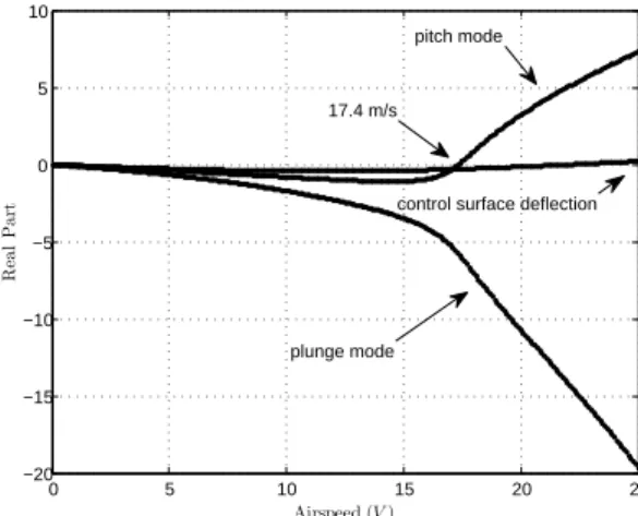
Considering δ = 0.0526 and ρ = 1.1638 kg/m3, let
1≤V≤25m/sandρtoρ(1+δ)be the flight envelope defined for this work. Figures 5 and 6 present frequency and damping plotted against airspeed for nominal system(ρ). Additionally, flutter speeds are identified as 17.4m/s and 17.0m/s, respectively for ρ and
ρ(1+δ) extracting the eigenvalues of the dynamic matrix. These reference results are used to show that this partially continuous method is able to identify stability regions in the flight envelope.
Application 1: Robust air density analysis
The stability analysis is performed according to the first approach (application 1) increasing∆V in 0.1m/sand also consideringρunc= 1.1638(1+0.0526)kg/m3. In the example N
Table 1. Physical and geometric properties of the 2D airfoil.
δ1=0.0526(5.26%) r¯β=
√ 0.00625
ρ=1.1638kg/m3 a=−0.4
M=5kg ωh=3Hz
b=0.15mandc=0.6 ωθ=5.5Hz ¯
xθ=0.2 ωβ=12Hz
¯
xβ=0.0125 β1=0.2β2=1.2β3=1.6β4=1.8
¯ rθ=
√
0.25 0.1≤k≤2.0;∆k=0.1
M−am1≈I−ρQm2+ρ2Q2m2 ⇒
M−am1=
0.9154 -0.0261 0.0176 -0.0288 0.9431 -0.0047 0.0073 0.0049 0.9863
I−ρQm2+ρ2Q2m2=
0.9165 -0.0256 0.0174 -0.0283 0.9435 -0.0048 0.0072 0.0048 0.9863
(27)
where its possible to note a good approximation for the inverse matrix. The convex spaceΩ∈R3is presented in Fig. 4 for whichv=3, rv=8 and the dynamic matrices are defined by
Ar1=A(δ
max
1 ,δ2min,δmin3 ) Ar5=A(δ
max
1 ,δ2min,δmax3 )
Ar2=A(δ
max
1 ,δ
max
2 ,δ
min
3 ) Ar6=A(δ
max
1 ,δ
max
2 ,δ
max
3 )
Ar3=A(δ
min
1 ,δmax2 ,δmin3 ) Ar7=A(δ
min
1 ,δmax2 ,δmax3 )
Ar4=A(δ
min
1 ,δ2min,δmin3 ) Ar8=A(δ
min
1 ,δmin2 ,δmax3 )
(28)
Note that the matrixArj defines therjth vertex based onρunc,ρ 2 unc,
ρ3uncandδ(j.), such that
ρunc=ρ(1+δ1) ⇒ δ1=∆ρρ | ∆ρ=δρ
ρ2unc=ρ2(1+δ2) ⇒ δ2=
ρ+∆ρ
ρ
2
−1
ρ3unc=ρ3(1+δ3) ⇒ δ3=
ρ+∆ρ
ρ
3
−1
(29)
Lyapunov inequality is solved for the range of interest of air density and the stability index is plotted against airspeed (Fig. 7). According to these results the system is stable for V <17m/s. Although a classical eigenvalue analysis indicates that the system is stable if V ≤16.5m/s, only this introduced approach is able to indicate stability over all continuous interval 1.1638≤ρ≤1.2250kg/m3for each velocity. In order to verify the
system stability in this flight envelope, only a complementary discrete analysis for each air density must be performed ifV >16.5m/s. Figure 8 illustrates the geometric region of analysis of the flight envelope for this novel approach. This continuous analysis overρ
toρ(1+δ) is an advantage mainly for flutter analysis in complex and large structures whose stability boundaries may be not easily predicted through discrete evaluation.
Application 2: Robust velocity analysis
0 0.01
0.02 0.03
0.04 0.05
0 0.05
0.1 0 0.05 0.1 0.15
δ3
Convex space (application 1)
δ1 δ2
Figure 4. Fictitious (parallelepiped) versus physical (line) domain.
0 5 10 15 20 25
2 4 6 8 10 12 14
16 2D Airfoil
F
re
q
u
en
cy
(Hz
)
Airspeed (V)
control surface deflection
pitch mode
plunge mode
Figure 5. Aeroelastic Frequency: 2D model (ρ=1.1638kg/m3).
0 5 10 15 20 25
−20 −15 −10 −5 0 5 10
Airspeed (V)
R
ea
l
P
a
rt
17.4 m/s
control surface deflection pitch mode
plunge mode
Figure 6. Real part of the eigenvalues (ρ=1.1638kg/m3).
0 5 10 15 20 25 −1
−0.5 0 0.5 1
Airspeed [m/s]
S
ta
b
il
it
y
In
d
ex
Air density range
16.5 m/s
Figure 7. Lyapunov stability index: application 1.
0 5 10 15 20 25
1.16 1.18 1.2 1.22
Airspeed [m/s] ρun
c
Air density range
Figure 8. Flight envelope discretization: application 1 (continuous range of
ρ).
Fig. 16 is obtained by performing a discrete analysis(∆V =0). If ∆V is large, a small number of analyses is required for evaluating the range[1,25]m/s. However, the aeroelastic stability region cannot be completely identified. Note that the mathematical domainΩcan result in not identifying the stability even at low speeds. This work does not propose criteria which should be used for choosing the optimal values of∆V.
0 5 10 15 20 25
−1 −0.5 0 0.5 1
Airspeed [m/s]
S
ta
b
il
it
y
In
d
ex
Application 2 : ∆V= 1.6m/s
5.8 m/s 12.2 m/s
Figure 9. Stability index:∆V=1.6m/s.
0 5 10 15 20 25
−1 −0.5 0 0.5 1
Airspeed [m/s]
S
ta
b
il
it
y
In
d
ex
Application 2 : ∆V= 1.5m/s
5.5 m/s 13.0 m/s
Figure 10. Stability index:∆V=1.5m/s.
0 5 10 15 20 25
−1 −0.5 0 0.5 1
Airspeed [m/s]
S
ta
b
il
it
y
In
d
ex
Application 2 : ∆V= 1.2m/s
3.4 m/s 13.0 m/s
Figure 11. Stability index:∆V=1.2m/s.
0 5 10 15 20 25
−1 −0.5 0 0.5 1
Airspeed [m/s]
S
ta
b
il
it
y
In
d
ex
Application 2 : ∆V= 1.0m/s
3.0 m/s 14 m/s
Figure 12. Stability index:∆V=1.0m/s.
0 5 10 15 20 25
−1 −0.5 0 0.5 1
Airspeed [m/s]
S
ta
b
il
it
y
In
d
ex
Application 2 : ∆V= 0.8m/s
2.6 m/s 13.8 m/s
Figure 13. Stability index:∆V=0.8m/s.
0 5 10 15 20 25
−1 −0.5 0 0.5 1
Airspeed [m/s]
S
ta
b
il
it
y
In
d
ex
Application 2 : ∆V= 0.2m/s
1.6 m/s 14.4 m/s
Figure 14. Stability index:∆V=0.2m/s.
0 5 10 15 20 25
−1 −0.5 0 0.5 1
Airspeed [m/s]
S
ta
b
il
it
y
In
d
ex
Application 2 : ∆V= 0.1m/s
1.5 m/s 14.5 m/s
Figure 15. Stability index:∆V=0.1m/s.
Conclusions
0 5 10 15 20 25 −1
−0.5 0 0.5 1
Airspeed [m/s]
S
ta
b
il
it
y
In
d
ex
Discrete Analysis
17.4 m/s −− unstable
Figure 16. Stability index obtained by computing a discrete analysis.
on a simple system have shown that this approach can be used to provide robustness in the flutter identification. Also, the paper has demonstrated that Lyapunov’s linear matrix inequality is a sufficient condition for verifying the aeroelastic stability.
Acknowledgements
The authors gratefully acknowledge CNPq for partially funding the present research work through the INCT-EIE.
Appendix
This appendix presents the submatrices introduced in Eq. (8).
A11=−Dm+ρV0.5bQm1−∑Nj=T1(−1)jρj 0.5b2Qm2 j
Dm
A12=∑Nj=T1(−1)
jρ(j+1)V 0.5b2Q m2
j
0.5bQm1
A1=A11+A12
(30)
A21=−Km+ρV20.5Qm0−∑Nj=T1(−1)jρj 0.5b2Qm2
j
Km
A22=∑Nj=T1(−1)jρ(j+1)V2 0.5b2Qm2 j
0.5Qm0
A2=A21+A22
(31)
A31=ρV20.5
h
Qm3···Qm(2+nlag)
i
A32=∑Nj=T1
h
(−1)jρ(j+1)V2 0.5b2Q m2
ji h
Qm3···Qm(2+nlag)
i
A3=A31+A32
(32)
A4= [I···I···I]T, (nlag+1)m×m | I, m×m (33)
A5= [0](nlag+1)m×m (34)
A6=V
−1 b
0 0 ··· 0
β1I 0 ··· 0
··· ··· ··· ··· 0 0 ··· βnlagI
, (nlag+1)m×nlagm
(35)
References
Albano, E., Rodden, W.P., 1969, “A Doublet-Lattice Method for Calculating Lift Distributions on Oscillationg Surfaces in Subsonic Flows,”
AIAA Journal, pp. 279-285.
Barmish, B.R., 1985, “Necessary and sufficient conditions for quadratic stabilizability of an uncertain system,”Journal of Optimization Theory and
Applications, Vol. 4, pp. 399-408.
Bisplinghoff, H.A., Raymond, L., Halfman, R.L., 1996, “Aeroelasticity,”, Dover Publications, INC.
Boyd, S., Ghaoui, L.E., Balakrishnan, V., 1994, “Linear Matrix Inequalities in System Control Theory,”Society for Industrial and Applied
Mathematics, Vol. 15.
Chen, P.C., 2000, “Damping Perturbation Method for Flutter Solution: The g-Method,”AIAA Journal, Vol. 38, pp. 1519-1524.
Chung, C., Shin, S., 2010, “Worst case flutter analysis of a stored wing with structural and aerodynamic variation,” AIAA Structures, Structural Dynamics, and Materials Conference, Orlando, Florida.
Chung, C., Shin, S., Kim, T., 2008, “A new robust aeroelastic analysis including aerodynamic uncertainty from varying Mach numbers,” AIAA Structures, Structural Dynamics, and Materials Conference, Schaumburg, IL.
Hassig, H.J., 1971, “An Approximate True Damping Solution of the Flutter Equation by Determinant Iteration,”Journal of Aircraft, Vol. 8(11), pp. 885-889.
Henderson, H.V. and Searle, S.R., 1981, “On Deriving the Inverse of a Sum of Matrices,”Society for Industrial and Applied Mathematics, Vol. 23, No. 1, pp. 53-60.
Lind, R., Brenner, M., 1999, “Robust aeroservoelastic stability analysis,”
Spring-Verlag, London, April.
Lyapunov, A., 1907, “Probleme general de la stabilite du mouvement,”
Annales Fac. Sciences Toulouse, Vol. 7, pp. 203-474.
Oliveira, M.C., Bernussou, J., Geromel, J.C., 1999, “A new discrete-time robust stability condition,”Systems & Control Letters, Vol. 37, pp. 261-265.
Pahlavanloo, P., 2007, “Dynamic Aeroelastic Simulation of the AGARD 445.6 Wing using Edge,”FOI - Swedish Defence Research Agency Defence
and Security, System and Technology.
Petersen, K. B. and Pedersen, M.S., 2008, “The Matrix Cookbook,”
http://matrixcookbook.com, Version November 14.
Roger, K., 1977, “Airplane Math Modelling Methods for Active Control Design,”Structural Aspects of Control, AGARD Conference Proceeding, Vol. 9, pp. 4.1-4.11.
Silva, S., Lopes Jr., V., 2006, “Active Flutter Suppression in a 2-D Airfoil Using Linear Matrix Inequalities Techniques,”Journal of the Brazilian Society
of Mechanical Sciences & Engineering, Vol. XXVIII, pp. 84-93.
Theodorsen, T., 1935, “General theory of aerodynamic instability and the mechanism of flutter,” Technical report 496, NACA – National Advisory Committee for Aeronautics.
Theodorsen, T., Garrick, I.E., 1940, “Mechanism of flutter A theoretical and experimental investigation of the flutter problem,” NACA – National Advisory Committee for Aeronautics.