J. Braz. Soc. Mech. Sci. & Eng. vol.34 número especial 2

Vincent Martin

CNRS vincent.martin@upmc.fr Institut Jean le Rond d'Alembert UMR CNRS/UPMC 7190

75005 Paris, France

The Fundamental Elements in Certain

Inverse Acoustic Problems: their

Roles and Interactions

Acoustic holography and holophony, wave field synthesis and active noise control are based on common elements which are causality, model, objective, and regularization. In the frequency domain (putting causality aside), a simple formulation states the influence – not the interaction – of errors of the model and objective and of regularization of the results. However, it does not give either an understanding or any relation of cause to effect. When the objective can be reached using the available model, regularization is not needed and the information liable to be extracted from this determined problem is poor, unlike in the over-determined case when the model does not allow the objective to be reached. The geometrical interpretation of the over-determined problem written in the least-mean square sense could be a tool to enlighten the influences and interactions in question. After having shown the interest of the geometrical interpretation, a pseudo-analytical inverse problem in spherical holophony and a numerical problem in plane holography provide particular illustrations. From among the properties accessible, one is highlighted: in the case of a perfect objective but inaccurate model, its adaptation brings a decrease in the amount of regularization required and an improvement in the results.

Keywords: inverse problems, regularization, acoustics

Introduction1

Acoustic holography (Metherel et al., 1967; Maynard, Williams and Lee, 1985, for the early works), wave field synthesis (Berkhout, de Vries and Vogel, 1993, for the early work), holophony, and active noise control (Nelson and Elliott, 1992; and Elliott, 2000, textbooks presenting a synthesis) are inverse acoustic problems sharing common elements such as causality, transfer function or model, objective or goal to be reached and regularization. In the frequency domain, the question of causality is put aside.

In these problems, one or a few sources are required to radiate a given acoustic pressure field (for an extensive overview of the past three decades with 170 references, see Wu, 2008). Indeed, sound field synthesis consists in determining driving signals to feed several loudspeakers in order to radiate a particular wavefront, a particular directivity in holophony; active noise control is linked to sound synthesis indirectly as the goal is to oppose a so-called acoustic primary field at the control microphone locations; holography is concerned with reconstructing a field in a whole domain from pressure measurements at a finite number of locations, this reconstruction often resting on the finding of the source strength at the origin of the measured field.

With less sources to control than given pressures to reach, the problem is overdetermined and rests on the least-square (LS) method, while with more sources than pressures leads to underdetermined problems with the least-norm (LN) method (the smallest solution from the infinity due to underdetermination, i.e. dealing with the LS method plus a constraint). Emphasized by Hald (2009), these solutions seem to coincide when regularization is involved. Limiting the investigation to overdetermined problems, the geometrical interpretation accompanies naturally the LS method with the Euclidian distance. The use of this interpretation has proved to be a good tool for investigating some properties such as the guaranteed quality of the procedure for reaching the objective (the given pressure field).

The geometrical view is also closely linked to the description of inverse problems with the vocabulary associated with sets, as presented by Kirsh (1996). For example, the given pressure field could be inaccessible for various physical reasons, all related to the pressure field not belonging to the set of fields the sources can generate. In active control, the secondary sources are not merged

Paper received 21 April 2012. Paper accepted 23 August 2012.

with the primary ones at the origin of the given pressure field and they cannot radiate the opposite field (except in the very particular 1D case of controlling plane waves in ducts); in holography primary and secondary sources are often the same, but here an erroneous measured field has no reason to be accessible. The best we can do is to reach the projection of the given field on the set of fields the secondary sources can radiate, leading to the geometrical point of view. The same will occur when the model is erroneous, and therefore, not liable to generate the objective. To generalize, it will be said that the model is not exact when incapable of radiating the exact objective (which does not mean that the radiation itself is erroneous), while the definition of an erroneous or an exact objective is kept natural.

So much for the objective space. Now what about the solution space (that of driving signals or source velocities)? To go from one space to the other, the model and its inverse are needed, and it is in the nature of things that the inverse of the direct operator is ill-conditioned (to the point that the differentiation between the two is through conditioning) which means that errors, whatever their reason for being, are greatly amplified in the solution and in the reconstructed field. The regularization acts on the inversion to limit the amplification and also plays a preponderant role in the spatial resolution of the solution obtained, as was underlined by Nelson and Yoon (2000), by Yoon and Nelson (2000), by Nelson (2001), by Kim and Nelson (2003). Regularization acts first in the solution space; in the objective space, only the consequences can be observed and this will be proved. Besides, we have noticed that the adaptation of the model to better radiate the perfect objective (the measured pressure without any errors) is accompanied by a need for less regularization and a better reconstructed field due to a better determination of the solution (driving signal or source velocities). This could help in finding the relation between solution and objective spaces through regularization and perhaps make use of the geometrical interpretation.

  far-field acoustic holophony and in nearfield acoustic holography illustrate the above properties. Open questions conclude this paper, devoted to an attempt to gather a variety of acoustic inverse problems with their uncertainties.

Nomenclature

a = scalar

a = vector

%

a = erroneous vector

n

a = nominal value of a

aopt or a_LS = least mean square solution obtained via the minimization of a functional; aopt is also for the case of optimality in general

A = matrix

%

A = erroneous matrix

* *

a , A = transpose conjugate of a, of A 1

−

A

= inverse of A

†

A

= pseudoinverse of A

a , A = L2-norm of a vector, of a matrix

δ

a

,

δ

A

= perturbation (variation) on a, on A

m

C = complex space of dimension m

min

d = minimal distance between two vectors in the L2 sense min

min

d = minimum possible value of d_min max

min

d = maximum possible value of d_min 1D, 3D = one-dimensional, three-dimensional

e = relative error on the objective

min

e = minimal relative error on the objective

E = transfer matrix or propagator F = efficiency of the inversion procedure h = Hankel function

I = identity matrix

m

I = identity matrix of dimensions mxm

J = functional made up of the square of the L2 norm of the distance between two vectors

0

J = initial value of J

att

J = part of J₀ the minimization procedure makes it possible to reach

res

J = residual part of J₀ after its minimization K = space of the image of the space of the source

velocities or control through the transfer matrix E

Log

= logarithm with base 10

LN = least norm

LS = least square

p

= vector of measured acoustic pressure at the microphones (objective vector)

,

n

p = projection of the exact nominal pressure vector to the erroneous nominal pressure vector

Q

= quality of the inversion procedure

g

Q = guaranteed quality of the inversion process

R = regularized matrix

m

R

= real space of dimension m

R

+ = space of positive real numbers Tr = trace of a matrix

v = vector of the source velocities or source controls

V

= space of source velocities or source controls

Y = spherical harmonics

β

= acoustic admittance

ε

= regularization coefficient

ψ

= angle between the objective vector and the hyperplane originating from the transfer matrix E

σ

= radiation efficiency

ϑ

= angle between the erroneous and the exact objective vectors

ANC

= active noise control

BIEM = boundary integral equation method

CSLA

= compact spherical loudspeaker array

ESM

= equivalent source method

NAH

= nearfield acoustic holography

SONAH

= statistically optimized nearfield acoustic holography

WFS

= wave field synthesis

Framework

The source or sources whose velocities are sought are called “secondary source(s)” to differentiate their role from the so-called primary source(s) at the origin of the radiated pressure. They differ in sound field synthesis, holophony and active noise control while they are merged in holography. Thus, in synthesis and control, secondary sources cannot radiate the primary field accurately in the whole 3D domain (contrary to cases related to 1D propagation).

As the primary field does not belong to the space of the fields liable to be generated by the secondary sources, it is said that the radiation model cannot be exact, with a clear sense in mathematical set terms. In contrast, there might be such an exact model in holography. Here a perturbed propagator, which is thus not exact, arises not from conceptual reasons but because physical data like sound speed, source and microphone locations are only approximated and/or because the measurements and calculations are not exact.

Concerning the objective, it is said to be exact if it perfectly describes the field to be generated. On a microphone array, it is necessary to have a sufficient number of sensors with a well-chosen distance between them according to the sound spectrum under study, and also strictly no measurement errors on the recorded and signal-processed pressures.

The above problems always rest on equation

=

p Ev (1)

where the vector p is the objective made up of the measured pressures at the M microphones of the antenna, the velocity or command vector v is sought at

N

points or on

N

sources, and E is the transfer matrix or propagator or model of dimensions M x N (M ≥ N) with rank E ≤ N. Quite often, the inverse problem is solved in the least-mean square sense to lead to the optimal velocity (or driving signals). Writing ₌ *

H E E, where the asterisk indicates the transpose-conjugate, we have:

-1 * ( , )

opt =

v E p H E p (2)

Very simple manipulations of Eq. (2) result in the perturbation

-

opt

δ

v

=

v

v

due to perturbation on the exact model E, on the exact objective p and on the numerical inversion of H. From now on, v is the exact vector solution.

Let us consider the perturbed model

E

%

=

E

+

δ

E

and the perturbed objective

p

%

=

p

+

δ

p

. As long as H% = E E% %* is perfectly invertible i.e., as long as the strict equality

-1

-

=

%

%

H H

I

0

holds, then _vopt( , ) _{E p% % = H E p%}-1_%*_%

according to Eq. (2). This leads to

δ

_v = _vopt( , ) - _{E p% % v} = _{H E%}-1_%*

δ

_p

(

+

_{H E Ev%}-1_%*

- )

_v

(3)

where H E%-1%* approximates the “inverse” of the rectangular matrix

%

E. Equation (3) is simple but with the drawback that it requires previous knowledge of E and v, making this equation uninteresting in the real world but a helpful first approach from the theoretical point of view. In fact Eq. (3) will become an equation about the error

δ

v when prior additional information on

δ

E and on

δ

p gives an upper bound.

When matrix H% is either not invertible or poorly inverted, because ill-conditioned, the pseudo-inverse H E%-1%* of E% is approached by a matrix R%_ε where the parameter

ε

can be adjusted to solve at best the problem while still avoiding unacceptable solutions. The matrix or operator R%_ε is called regulator, the most famous being that of Tikhonov. If the numerical calculation error is negligible, we have:

( , ) - ( ) - ( - )

opt

ε

ε ε

δ

δ

δ

= = +

= +

% _% %

% %

v v E p v R p p v

R p R Ev v (4)

which is similar to Eq. (3).

How Ev% opt tends towards

p

or

p

%

or, when a calculation is carried out with the adjusted value of

ε

named

ε

opt, how opt

opt ε

%

Ev tends towards

p

or

p

%

or how

ε

opt depends on

δ

p

or

δ

E

, are the questions addressed in this paper.

The geometrical interpretation of the inverse problems dealt with previously by the author could constitute a tool to contribute to answering the questions.

Geometrical Interpretation

The raw material of this section is to be found in Martin and Cariou (1997), in Le Bourdon (2009), and in Martin, Le Bourdon and Arruda (2012).

Inverse problem and projection

In presence of perturbation on the objective and on the model, solution vopt( , )E p% % in Eq. (2) results from the algorithm

2 min ( ) min

v

J = % − %

v v Ev p (5)

with the L2-norm in the objective space. This Euclidian (Hermitian norm in the complex field) norm leads naturally to a geometrical

point of view as this operation can be seen as the projection of the objective

p

%

on the hyper-plane spanned by the columns vector of matrix E%. The minimization leads to the minimal distance

min( , ) opt

d E p% % = Ev% −p% which is the square root of the residual part J_res of

J

after the operation. Let us define J₀as the value of

J

when the velocity is zero, that is J₀= p% 2 and J_att=J₀−J_res the part of

J

that has been attained thanks to the calculation of

opt

v

. It appears that J_att= Ev% opt 2. These definitions allow us to read symbolically the projection operation in Fig. 1 where the objective does not belong to the hyper-plane due to a perturbation in

p

, in E, or in both. In these conditions there exists a non-zero angle

ψ

%

(written

ψ

for the exact

p

) such that

_sin

ψ

_%=dmin( )%

%

p

p , (6)

differing from the general cross-validation parameter defined as (see Hansen, 1998):

2 min 2

( *)

d

Tr I−EE% % .

The efficiency is defined by

2

2 ( ) cos Jatt

F % =

ψ

%=

%

p

p . (7)

Therefore, given

p

%

and E% , the die is cast for the optimal value of the velocity and for the efficiency. To improve the efficiency there is no choice but to reduce angle

ψ

%

(through d_min) hoping to better approach the true value v under some assumptions. This angle has proved to be efficient for classifying various propagators (transfer matrices) in the automotive industry by Le Bourdon, Picard, Martin (2009).

Error of the objective

In general, the vector of the acoustic pressure is measured data and, for this reason, inevitably erroneous, while being the only data available. It is said "of reference" or "nominal" and written p_n. The true pressure

p

is somewhere around this nominal value and is of the form p=p_n+

δ

p. For the time being and for the sake of general notation let us write p%_n=p_n+

δ

p with p%_n seen as a perturbed field relatively to p_n, underlining that the unknown true pressure results from a variation in the available nominal pressure.

The error in the objective is defined by

( ) n n

n

n

e p% = p% −p

  and p% = J0

min res d = J

ψ% ψ % p opt % E v

space originating from E%

and E v% opt = Jatt

Figure 1. Projection operation related to the minimization of functional J.

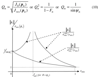
As emphasized by Martin and Gronier (1998) and by Martin, Le Bourdon and Arruda (2012), this quantity may constitute a vicinity around the reference field containing all the perturbed fields such that their relative error is less than or equal to a given value of e. Ideally, a vicinity around p_n should correspond to a vicinity around the efficiency F_n=F(p_n) in order to establish a connection between efficiency and error in the objective and, by so doing, to be able to see how the efficiency diverges from that of reference when the error in the reference field increases. In fact, the previous definition of the vicinity around p_n, expressed by e, is such that to a given efficiency corresponds an infinite number of different values of e spread over the interval [0 ,+ +∞(. Indeed the efficiency defined by the angle

ψ

%_n associated with p%_n is the same for an infinite number of collinear fields p%n, and, therefore, to an infinite number of values of e(p%_n). On the contrary, for all these collinear fields sharing the same efficiency, a single minimum value belonging to interval [0,1]was defined by Martin and Gronier (1998). The following definition is thus preferred:

* 2 min . ( ) n n n n n n n e − = % % % % p p p p p p

p (9)

Moreover it has been shown that a given value of e_min corresponds to a single value of the guaranteed efficiency when the perturbed field p%_nbelongs to the vicinity defined by e_min.

It appears that e_min is the sinus of angle

θ

shown in Fig. 2 and therefore, is a measurement of the aperture of the cone centered on the reference objective (Fig. 3).

min( n)

d p n

ψ

n p space originating

from E%

n′ % p n % p θ

min( n)

d p%

min( ' )n

d p%

Figure 2. Angle

θ

related to .

n ′ p%

min( n)

d p n ψ θ n p min min min( )

d e

max min min ( )

d e

space originating

fromE%

min( n)

d p%′

n p%

Figure 3. Cone related to defining a vicinity of the given nominal field .

A point of coordinates _min

min ( ), ( ) n n n e d       % % % p p

p can be associated to each perturbed field in the vicinity of the reference

field . Let us notice that

' ' min( ) min( )

n n

n n

d =d

% %

% %

p p

p p where is the

projection of on . For a set of perturbed fields sharing the same minimal relative error, the values d_minmin(e_min) and

max min( min)

d e (see Fig. 3) bound the range of dmin(p%n')for any field considered in that set. Figure 4 illustrates the theoretical result.

Guaranteed quality of the inverse process in the objective space

For a given reference objective , the reference or nominal quality of the process is defined by the quantity

0( )

( ) n n res n J Q J = p

p or

2 1 1 n n Q F =

− or

1 sin n n Q

ψ

= (10)

( )

' ' min n n d % % p p ( ) ' max min min n d e % p ( ) ' min min min n d e % p min e 1 0 1 1 sinψn

min( n) eθ forθ ψ=

Figure 4. Theoretical form of the bounds of the cloud of points

(

emin(p%n), p%n /dmin(p%n)

)

.

the geometrical representation, p_n' is the projection of the reference pressure on the edge of the cone located farthest from the model hyper-plane, the quality of inverse process is always better than that defined by

0( ') ( ')

n g

res n

J Q

J

= p

p , (11)

said to be the guaranteed quality. Therefore, it is straightforward that the guaranteed quality is given by

2

min min

1 1

sin( ) sin cos cos sin

1

1 1

g

n n n

n n

Q

e F e F

θ ψ

θ

ψ

θ

ψ

= =

+ +

=

+ − −

or

2 2

min min min

1

1 (2 1) 2 (1 ) (1 )

g

n n n n

Q

F e F e e F F

=

− + − + − −

.

(12)

Equation (12) was found by Martin and Gronier (1998) but via an analytical approach far more complicated than this simple geometrical way. The analytical demonstration is still interesting but no longer as for the result more directly obtained today.

Graphs showing, in logarithmic scale, the guaranteed quality against the reference quality for various values of e_min are given in Fig. 5. The main point here is that the graphs present a plateau for high nominal quality leading us to conclude that, for a given value of e_min, an increase in the nominal quality is not rewarded by a significant increase in the guaranteed quality. When the nominal quality is obtained by adapting a model to make the hyperplane of draw nearer to , this information gives the limit of the effort beyond which there is no need to go further.

Figure 5. Guaranteed quality against nominal quality for various errors in the objective.

It has thus been shown in this section that the geometrical interpretation has proved to be a useful tool for presenting the guaranteed quality of the process of inversion, and also to reveal a cost function for adapting the model. However this tool operates only in the objective space.

Model Adaptation versus Regularization: Observations, Generalization, Difficulties

When the model and/or the objective is/are not exact, there is a need for regularization such as Tikhonov's or of another type, for example by discarding the small eigenvalues of the propagation matrix. When only the model is not exact, the operation of adapting the model consists in reducing the angle

ψ

to the exact objective. Thanks to case studies, it has been observed on the one hand that the regularization has no effect on

ψ

and on the other hand that the smaller the angle

ψ

, the less optimal regularization needed and the better the results. While we have found a demonstration for the first observation, there is still research to be done to find how regularization and errors are related.

Error of the objective and of the model

In very general terms and before speaking of exact or perturbed objective and model, the question is to see if the writing of

Ev

=

p

is meaningful and if there is a solution. Let

V

be the solution space and let K be the image of

V

through the model E:

E

(V)

≡

K

.

When

p

∈

K

, the writing

Ev

=

p

is meaningful and the LS solution LS ( * )1 *

−

=

v E E E p leads to the exact valuev. Indeed

1 1

( * ) * ( * ) *

LS

− −

= = =

v E E E p E E E Ev v.

When

p

∉

K

, the writing Ev = p has no sense for

v

∈

V

(if

V

∈

v

, then

p

∈

K

) and either v exists outside

V

, or it does not exist. If the LS solution LS ( * )1 * V

−

= ∈

v E E E p , it would

generate

p'

∈

K

, necessarily different from

p

. When

p

∈

K

but

(V)

≡

K'

E

where

p

is not located, the same remark can be made. In the case of errors in the objective only, the problem to solve is more precisely written

Ev

=

p

%

which has no sense as it is unlikely for

p

%

∈

K

. For a well-conditioned matrix H the optimal solution vopt( , ) E p% = H E p-1 *% differs from the exact solution v associated with the exact pressure by

-1 * ( , ) -

opt _{% =}

δ

v E p v H E p (13)

as stated by Eq. (3) with E in place of E% . When H is ill-conditioned the regularized Tikhonov solution is

1

( * ) *

opt

ε = +ε − %

v E E I E p (14)

which differs from the exact solution by

(

)

1 1

( * ) * ( * ) *

opt

ε − =

ε

−

δ

+

ε

− −

v v E E + I E p E E + I E p v (15)

in conformity with Eq. (4) with Ein place of E%.

In the case of errors in the model only, the problem to solve is written Ev% = p. The regularized Tikhonov solution is

1

( * ) *

opt

ε = % %+ε − %

v E E I E p (16)

  1

( * ) *

opt

ε − = % %+

ε

− % −

v v E E I E Ev v (17)

It is clear that if there exists, when

E

%

→

E

(in a sense to be defined), an optimal value

ε

optof

ε

that tends towards zero in

R

+, then v_εopt→v (in a sense to be defined). So far, the adaptation of the model carried out to obtain

E

%

→

E

rested on the minimization of angle

ψ

. And, effectively, the process was accompanied by the observation of

ε

opt

→

0

. It was tempting to assume that the regularization modified the model in order to reduce

ψ

. The observation countered this assumption and we demonstrate below in four steps the independence of angle

ψ

from the coefficient

ε

with the consequence that the effect of regularization cannot be described easily in the objective space (Martin and Le Bourdon, 2010), perhaps a natural conclusion in retrospect since E% is not acted upon, contrarily to its "inverse" H E%−1%* now written E%†.

Independence of the angle

ψ

from

ε

Without jeopardizing generality, suppose only the model is not exact.

1. Let us consider min ( )J =min % 2 v v v Ev - p

with

: n ( ) m

V⊂C → V = ⊂K C

% %

E E and J C: n→R+ where m>n. The space

V

could contain for example only those variables the norms of which are bounded by a given maximal value. With in place of , Fig. 1 above has given the Euclidian representation with

2

V⊂R and 3

( )V = ⊂K R %

E , and in the case where p∉E%( )V . The singular value decomposition (SVD) of E% is such that

{ { { { , , , , * n n m n m m diagonal

m n =

%

E U ΛΛΛΛ V with U U* =UU*=I and m V V* =VV*=I . n

Matrix ΛΛΛΛ is diagonal in its upper part and zero in its lower part. Matrix U is made up of base vectors of the objective space where the data p is located, and matrix

V

is formed with the base vectors of space V of variable v . When p∉E%( )V , one cannot find

V ∈

v (one cannot invert E%) and _%−1

E is replaced by the term called pseudo-inverse of E% that is _{

(

)

1_{

, , , † n m n m n n * − * = % % % %

14243

E E E E . This operation

leads to the solution vopt∈V such that it generates the nearest '∈ ( )V =K

p E of p in the sense of the Hermitian norm in . As opt_{= %}†

v E p , it results in opt † *

=

v V

Λ

ΛΛ

Λ

U p with

{

( )

{ 1 † * , , , n m n m n n * − =

14243

Λ Λ Λ Λ

ΛΛ Λ Λ ΛΛ Λ Λ

Λ Λ Λ Λ . We have also _{† , 0 0 0 n m m =_ _   ΛΛ ΛΛΛΛ

ΛΛ I leading to

(

)

† † * opt * * = = % %

Ev EV

Λ

Λ

Λ

Λ

U p U VΛΛΛΛ V

Λ

Λ

Λ

Λ

U p or

† 0 0 0 n opt * * = = _ _   % I

Ev UΛΛΛΛ

Λ

ΛΛ

Λ

U p U U p.

2. Now let us consider the functional of Tikhonov which helps in approximating the inverse matrix _%−1

E and is a regularization process: Jε( )v = Ev - p% _K2 +ε v_V2 with

: n

J_ε C →R+ and ε∈R+.

For a given ε, opt † *

ε = ε

v V

Λ

ΛΛ

Λ

U p arises from minimizing ( )

J_ε v with †ε

(

* ε n

)

1 *

−

= Λ ΛΛ ΛΛ ΛΛ Λ+ ΛΛΛΛ

Λ

ΛΛ

Λ

I .

3. Let us write E%_ε =UΛΛΛΛ_εV* not yet having defined ΛΛΛΛ_ε (but the access to which is not difficult) and let us consider

2 '

( )

J_ε v = E v - p%_ε , the minimization of which for a given ε

provides ' opt

ε

v . It appears ' opt opt

ε = ε

v v . So, for the time being, functionals J_ε( )v = Ev - p% 2+ε v and 2 J_ε'( )v = E v - p%_ε 2 share the same objectivep and the same optimal value of their variables.

4. But we have

(

)

' † * 0 0 0 opt opt n opt * *

ε ε ε ε

ε = = ε

= _ _ =

 

% %

%

E v E v U V V U p I

U U p Ev Λ

ΛΛ Λ

Λ

ΛΛ

Λ

.

In these conditions, functionals J( )v = Ev% −p 2 and

2 '

( )

J_ε v = E v%_ε −p share the same objective and the same minimal distance dmin and this whatever ε. Therefore angle ψ such that

' cos

opt opt

ε ε

ψ = Ev% = E v%

p p does not depend on the Tikhonov coefficient ε. In the case of the Euclidean configuration shown in Fig. 1 this is true for both functionals.

5. Finally, the Tikhonov regularization does not seem to have an influence on angle ψ in space of the objectives, but it plays a role in space V of the solutions. Therefore, we cannot expect to represent easily (if indeed it is possible) the regularization process in the objective space.

Optimal regularization and illustration on a simple example

Going back to opt( , )

ε %

v E p , let us notice that, when solving

0 min opt

ε

ε≥ v −v with the 2

L

-norm in the solution space, the results observed in examples (therefore without generalization yet) is

0

opt

ε

= whatever

δ

E

and therefore,

v

_εopt

−

v

cannot be used for finding

ε

opt(leaving aside that v is not known). Were we to accept negative values of

ε

, there could be a value to make

opt

ε

−

v

v

zero. Indeed 1

( * ) *

opt

ε − = % %+

ε

− % −

v v E E I E Ev v = 0 when E%*Ev=(E%*E%+

ε

I v) i.e.

E

%

*

δ

E v =

-

ε

v

. This can be true only if

E

%

*

δ

E v

is collinear with v, a very strong constraint. Its LS value would be εLSopt ( * ) 1 * ( * δ *)δ

−

= − v v v E + E E v

where it is true that the dependence on

δ

E

is made explicit, but this value does not minimize v_εopt−v and moreover, what has been observed concerns

ε ψ

opt( ), not

ε δ

opt( E).

opt

Log v_ε against Log Ev% _εopt−p (Kirsh, 1996; Hansen, 1998). The optimal value

ε

opt corresponds to the compromise located at the “corner” of the

L

-curve where the curvature is maximum. However, the idealized

L

-curve has not always so clear a form and the location for obtaining

ε

opt should be determined with care.

Let us say that

ε

opt has been defined by Steiner and Hald (2001), as depending on the signal to noise ratio (SNR) seen at the objective and due to all sorts of reasons (measurements, errors in the model, calculation approximations). The SNR is defined by rule of thumb and is not seen as model dependent. However, Hald (2003) wrote with the present notations that “re-scaling of the matrix

*

% %

E E in turn necessitates a re-scaling of the regularization parameter

ε

opt”. And again to emphasize the state of the art concerning the dependence of

ε

opt on the model, let us refer to Gomes and Hansen (2008) where, according to the type of model chosen – which could be that of Statistically Optimized Nearfied Acoustic Holography (SONAH) to replace the first version of NAH from Maynard et al. (1985), or that of the Boundary Integral Equation Method (BIEM) as developed by Bai (1992) or described by Augusztinovicz and Tournour (1999), or that of Equivalent Source Method (ESM) – , there is a change in the best regularization parameter. The work of Gomes and Hansen is an echo of the earlier work carried out by Williams (2001).

0.2 0.4 0.6 0.8 1.0 1.2 1.4 0.2

0.4 0.6 0.8 1.0 1.2

opt

LogEv% ε −p

opt Logvε

0.2 0.4 0.6 0.8 1.0 1.2 1.4 0.2

0.4 0.6 0.8 opt

Logv_ε

opt Log Ev%_ε −p

Figure 6. Two types of L-curve for the numerical example dealt with.

Is the observation concerning the decreasing of

ε

opt with that of

ψ

made when solving physical inverse problems closely linked to the underlying physics, or is it a more general property? To try to answer that question, let us take a very arbitrary matrix

1. 2.

1.1 2.1 5. 6.

 

 

=_{ }

 

 

E and an arbitrary perfect velocity 7. 12. −

 

= 

 

v . In

these conditions, the perfect objective is

17. 17.5

37.

 

 

= 

 

 

p . Let us

perturb the term (1,2) of E to obtain E% with a law such that 1,2 1,2(1. 0.5 [ 1, 1])

E% =E + Random Real,− + , i.e. with unstructured uncertainties. First, calculate the angle

ψ

(calculated through

sin

opt

ψ

= Ev% −p

p ) , then draw the

L

-curve, and in the case of a relatively visible “corner”, find the

ε

opt, and finally calculate

opt opt

ε −

v v . It must be said that the value of

ε

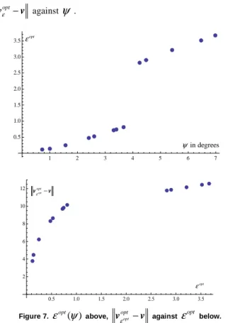
opt retained is such that the quantity (Log Ev% εopt−p)2+(Log vεopt )2 is minimal, which is never far from the maximum curvature but not always at exactly the same location. Figure 6 shows two types of

L

-curve retained during the process and Fig. 7 shows

ε ψ

opt( )

, and opt

ε −

v v against

ψ

.

1 2 3 4 5 6 7

0.5 1.0 1.5 2.0 2.5 3.0 3.5

in degrees

ψ

opt

ε

0.5 1.0 1.5 2.0 2.5 3.0 3.5 2

4 6 8 10 12

opt ε opt

opt ε −

v v

Figure 7.

ε ψ

opt( ) above, opt opt

ε −

v v against

ε

opt below.

This simple numerical experiment shows that the decreasing of opt

ε

with

ψ

and that of opt opt

ε

−

v

v

with

ε

opt could be a general

Beyond the observation made on this very simple calculation experiment, how can it be demonstrated that opt

opt

ε

−

v

v

decreases

with the angle

ψ

? What are the difficulties? Indeed, let us write

1 * 1 * 1 *

1 * 1 * 1 *

opt opt

opt opt opt opt opt opt

( ) ( )

ε ε

ε

ε

− − −

− − −

− = − + −

= − + −

≤ − + −

% % % % %

% % % % %

v v v v v v

R p H E p H E p H E p

R H E p H E H E p

(18)

where it can be demonstrated (via the SVD of E) that

1 * ₀

(R%_ε−H E%− % )p → when

ε

→

0

, where it is natural that 1 * 1 *

0

(H E%− % −H E− )p → when (H E%−1%*−H E−1 *)→0. But how can the dependency on

ψ

be expressed? To this end, the

expression of

ε ψ

opt( )

will be needed. By accepting that

ε

opt is the

solution of min (Log _εopt )2 (Log _εopt )2

ε Ev% −p + v , the expression

in terms of

ψ

such that sin

opt

ψ

= Ev% −p

p does not seem an easy task.

While the following case studies as well as the above calculation example have shown that the adaptation of a model using the parameter

ψ

could be an interesting direction to follow, the definitive interest ought to depend on the demonstration sought and this question seems to be still open.

Case Studies

Semi-analytical spherical holophony in the far field

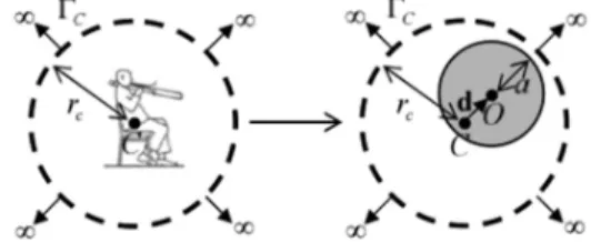
In Pasqual and Martin, 2012, a primary field due to a source (or sources) in a sphere Γ_c of centre C is given on the spherical surface

c

Γ (Fig. 8). This area is located in the far field relative to the source. The given pressure is expanded in a series of P independent functions composed of spherical harmonics considering the coordinate center O. The number of « modes » to describe the primary pressure with a good approximation depends on the coordinate center O. The minimum value of P occurs when O is at the so-called acoustic centre, in general unknown, even when the geometrical centre of the primary source is given.

A secondary source is required to radiate the given primary pressure as well as possible. This source, within the sphere but also far from its surface, is constrained to radiate a controllable given number S of « modes » with

S

≤

P

; some of them not radiating efficiently, leaving

S

'(

<

S

)

efficient controllable modes.

Where should it be located to reproduce the primary field as well as possible? The problem is equivalent to that of finding the location of the secondary source centred at O. It should be said that the problem of reproducing a field by a spherical source has also been investigated by Peleg and Rafaely (2011).

We are facing an inverse acoustic problem where the model of the secondary radiation has to be adapted through the secondary source location to reproduce at best the primary field. Due to the secondary source constraints, there are

P S

−

'

« modes » missing to reach the goal, a number that depends on O. Often, but not always, the minimal difference occurs when O is at the acoustic

centre of the primary source(s). This difference

P S

−

'

will play the role of regularization.

Figure 8. Illustration of the exterior spherical acoustical holophony.

The primary harmonic pressure is developed in the form

0

( / ) ( ) ( ) ( , )

P N n

p nm n nm

n m n

p O C h kr Y

θ ϕ

= =−

=

∑ ∑

x d (19)

where h_n are the Hankel functions and Y_nm are the spherical

harmonics. There are P=(N_p+1)2 terms; however, the axisymmetry of the pressure field reduces the number of terms to

( _p 1)

P= N + as

m

=

0

. For example, the field shown in Fig. 9 is such that there is a need for

n

>

1

to radiate it, whatever O (i.e.,

3

P

≥

). The coefficients C_nm can be determined almost exactly

∀

d

providing N_p is sufficiently large. In the example chosen,

6 p

N = , therefore

P

=

49

in general and

P

=

7

here. In other words, the number of modes with non-zero (or negligible) coefficients depends on the location of point O.

Figure 9. Axisymmetric primary field on Γ_c. The shape and the color map indicate, respectively, the amplitude and phase (in degrees) of p x_p( _c).

1

( / ) t( ). .

p p

p x O =s x H−

γγγγ

(20)

These new coefficients make up the spherical wave spectrum of the primary pressure evaluated at Γ_c.

The identification of

γγγγ

_p leads to their value

γγγγ

ˆ_pand, in the present situation, Pis sufficient to ensure a good if not exact reconstruction of p_p( /x O), whatever O.

Similarly the secondary harmonic field is expressed by

0

( / ) ( ) ( , )

S N n

s nm n nm

n m n

p O D h kr Y

θ ϕ

= =−

=

∑ ∑

x (21)

written

1 ( ) t( ). t( ). .

s s

p x =s x d =s x H−

γγγγ

(22)

Simply enough, our goal would be perfectly achieved with ˆ

s= p

γ

γ

γ

γ

γ

γ

γ

γ

if the secondary source were located at the acoustic centre of the primary source and able to radiate

S

=

P

modes. However, the secondary source constraints with

S

<

P

have been mentioned and moreover, from among the

S

modes, a number do not radiate efficiently.

Indeed, the radiation efficiency of a compact spherical loudspeaker array (CSLA) has the form shown in Fig. 10. Asking of such a source to radiate in the low frequency range with a large n leads to far too high a level of driving signal or velocity. It was decided to discard these disturbing high values of n and consider only those n associated with a reasonable minimum value

σ

_minof the efficiency. To illustrate, working with ka = 0.3 and considering only those modes with

σ σ

> _min=10−5, only

n

=

0

and

n

=

1

are left, therefore, N_s =1 and

S

=

4 or 2 for axisymmetric pressure distribution. Let us recall that 3

≤ ≤

P

7in the case studied. It appears that 4 sources of the CSLA, placed at the so-called extremal points for hyperinterpolation distributed over the spherical box can be driven to radiate efficiently 4 modes (and 2 sources for 2 modes).

Figure 10. Radiation efficiency curve for a spherical source with radius a for n≤3.

This discarding plays the role of the regularization as it facilitates access to the solution of the inverse problem, and the best solution in the LS-sense for ( ) t( ). 1.

s s

p x =s x H−

γ

leads to ,

s= s regul

γ

γ

γ

γ

γ

γ

γ

γ

in the following way:

, min

, ,

min 0

s i n s regul i

n

if

if

γ

σ

σ

γ

σ

σ

≥



=

<

 (23)

Let us define the regularization quality factor

λ

by

, ˆ

1 ˆ s regul p

p

λ

= −

γ

γ

γ

γ

−

γ

γ

γ

γ

γγγγ

(24)

which is the inverse of the amount of regularization. Clearly, when

, ˆ

s regul→ p

γ

γ

γ

γ

γ

γ

γ

γ

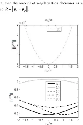
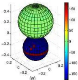
thanks to seeking the best location for the secondary source, then the amount of regularization decreases as well as the residue R= p_s−p_p .

Figure 11. Norm of the optimal radial velocity without and with regularization by discarding. Results as function of for the primary field shown in Fig. 9. Only the graphs are considered in this paper.

regularization quality factor as functions of z_s(only graph e is of interest here). It appears that R z( _sopt)>0 because the primary field cannot be accurately decomposed into spherical harmonics of order

1

n

≤

. However R is greatly reduced if the secondary source is placed at the optimal location.

Figure 12. Above, normalized residual norm

R z

( ) /

_s

p

_p

(

x

_c

)

and below regularization quality factor function of (primary field in Fig. 9). Graphs are considered in this paper.

Figure 13. Sound pressure field produced by a spherical secondary source placed at the optimal position for reproduction of the primary field in Fig. 9. The shape and color maps indicate respectively the amplitude and phase (in degrees).

The results presented show, in an almost natural way, that the adaptation of the model (here through the source location) is accompanied by a reduction in the regularization needed and improves the reconstruction. The synthesized field is given in Fig. 13.

Numerical nearfield holography

In Martin, Le Bourdon and Pasqual (2011), a thick vibrating disc (Fig. 14) radiates sound in the unbounded 3D space. The acoustic pressure is measured on a plane array of microphones parallel to one side of the disc, called the front face.

From the inverse procedure called here holography, the type of vibration on the front face is deduced from the measured pressure at the microphone array. It is supposed that the disc is embedded in a total front plane made up of Γ₁ and its complementary part Γ₁c.

How to take into account the radiation behind this front plane due to the vibration of the rear face and the thickness? This problem originates from the acoustic holography of a rolling wheel embedded in a car body. Despite the slightly different goals, let us quote the work of Schuhmacher et al. (2003), on a quite similar subject.

Ω

z

y

x

v r

2 2 2

Γ = Γ ∪ Γ

r v

1 1 1

Γ = Γ ∪ Γ

3 Γ

0

Figure 14. A thick disc, with vibrating front face Γ₁, rear face Γ₂, thread

3

Γ , radiates in the unbounded 3D space Ω.

Presently the radiation model is obtained through the boundary integral method that has the continuous form

1

1

1

1 2

1 1

2

1 1

2

( ) i ( ) ( , ) d

i ( ) ( , )d

i c ( ) ( , )d c

p Q v P g P Q P

k p P g P Q P

k p P g P Q P

ρ ω β β

Γ

Γ

Γ

=

+

+

∫

∫

∫

(25)

leading to the discrete form

(

-1

)

1 1 1 1

( , ) - ( , )

t c c t

p = i

ρω

ikc

β β

_I ikA

β β

_ B+ d v

or p = (E

β β

₁, ₁c)v (26)

where

β

₁ and

β

₁c are the unknown admittances (in a particular sense) respectively on Γ₁ and Γ₁c.

For the numerical simulation, the given modal forms on the faces and on the thickness are

( )

( )

(

)

( )

min

max min

-, sin cos -

- 2

, sin cos

i

i

r r

v r a l

r r

y

v y a l

e

π

θ θ π

θ θ π

 

=  

 

 

=  

 

(27)

Admittances

β

₁ and

β

₁c are local reactions and depend on the

point

x

∈ Γ

_s. Therefore, there are an infinite number of variables to identify and it is impossible to find the true propagator in these conditions. However, it has been observed that the admittance on

s

unknowns in the propagation model is directly linked to the number of points in the meshing of the source plane. It appears unrealistic for computation time reasons to identify each local admittance. To reduce the number of unknowns, the admittance is approached by a known function based on its expected form, and now only a small number of coefficients of the function must be identified. In the case of the thick disc, the following approximation

β

%

has been chosen:

(

)

(

)

[

]

[

(

5 2

8 10

1 3 4 6 max

7 9 max

e i e 0,

i ,

c r c r

c c

c c c c r r

c r c r r r

β

= + + + ∀ ∈

+ ∀ ∈ +∞



% ₍₂₈₎

where the coefficients c_{i i( 1,10= )}∈R. Adapting the propagator consists now in identifying the 10 coefficients. However this simplification is at the price of information about the function.

Using the genetic algorithm with the cost function made up of the angle

ψ

, the coefficients have been obtained approximately and the results are given in Fig. 15.

Figure 15. Admittance on the front face, expected and reconstructed.

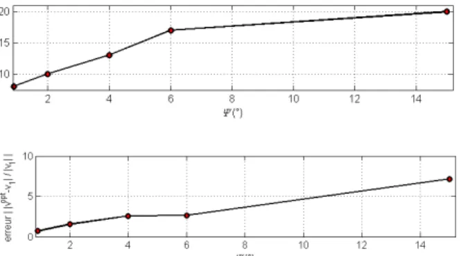
Figure16: Optimal Tikhonov regularization parameter and error in the reconstructed velocity versus the cost function.

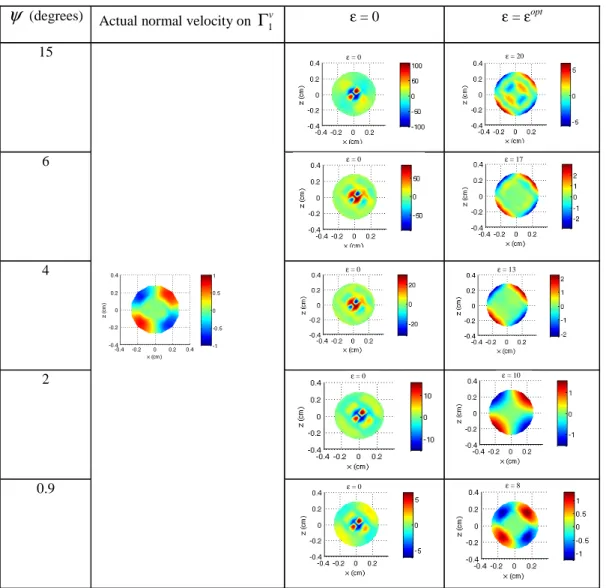
Table 1 shows the vibrating form obtained for the front face and Fig. 16presents the same results in another form, namely the optimal value of the Tikhonov regularization parameter against angle

ψ

, itself depending on the admittance on the front face

1 1

c

Γ ∪ Γ , as well as the error in the reconstructed velocity against angle

ψ

.

These results illustrate again the interaction between the adaptation of the model and the value of the regularization parameter with the consequence on the reconstructed velocity.

Conclusion and Open Questions

The present paper has given very general equations linking errors in models as well as in objectives and errors in the solution of certain inverse problems. Some interactions between models, objectives, errors, and regularizations are not visible in these equations while their consequence on the solution is well described. The current research attempts to contribute in finding the actions and interactions at play.

The geometrical interpretation has proved useful to show very easily the guaranteed quality of the inverse procedure, and also to define a cost function (angle

ψ

) to adapt the model in cases where the objective is exact. It has been demonstrated that the regularization does not act on

ψ

in the objective space (it acts in the solution space) and that a smaller cost function leads to a lesser optimal regularization parameter and gives a better solution. These links have been seen in a very simple calculation example outside all physical meaning. However no demonstration has yet been found.

The question of error in the objective with an exact model has not been addressed here, except through the guaranteed quality. Nevertheless angle

ψ

exists for an exact model and a perturbed objective. However, the aim here, not worked on yet, is to adapt the pressure to reach the model, not the opposite.

Now it must be underlined that the adaptation of the model has been carried out via the reduction of angle

ψ

from the exact objective. In the presence of perturbation on the objective, the same procedure would be followed by reducing angle

ψ θ

+

without being able to distinguish

ψ

from

θ

. If the adaptation works well, the model will reach the perturbed objective and thus be far from the exact objective by angle

θ

. If

θ ψ

>

, the cure is worse than the disease! How should the problem, clearly defined in geometrical terms, be tackled?

Another question concerns the geometrical representation of the best location of the sensors and their robustness. It was at the center of preoccupations in active control in the 2000’s, as the paper by Baek and Elliott can testify. In this field, Martin and Gronier (2001) showed, first, that it is always possible to obtain the nominal quality of the inverse process by filtering a small number of components of the reference objective and, second, that the robustness of the filtered sensor configurations was not identical. It could be that the first property may be understood thanks to geometrical representation in the objective space (moreover with an understanding of one of the constraints associated with the assertion) and that the robustness may be understood by looking in the direction of the projection of the cone on the subspace to which the filtered components of the objective belong.

Acknowledgements

The author thanks J.R. Arruda, Professor at the University of Campinas, Brazil, and R. Sampaio, Professor at the Pontifical Catholic University, Rio de Janeiro, Brazil, for the interest they showed to the present work.

References

Augusztinovicz, F., Tournour, M., 1999, “Reconstruction of source strength distribution by inversing the boundary element method” in O. Von Estorff (Ed), Boundary Elements in Acoustics: Advances and Applications, The Bristish Library, The world’s knowledge, pp. 243-284 (Chapter 8).

Baek, K.H., Elliott, S.J., 2000, “The effect of plant and disturbance uncertainties in active control systems on the placement of transducers”, Journal of Sound and Vibration, 230(2), pp. 261-289.

0.2 0.4 0.6 0.8 1 1.2 1.4 1.6 1.8

-0.25 -0.2 -0.15 -0.1 -0.05 0 0.05 0.1 0.15 0.2 0.25

r (m)

β

actual β_R actual β_I β_Ropt

Table 1. The vibrating form obtained for the front face of the disc without regularization and with optimal Tikhonov regularization

versus the angle

ψ

playing the role of the cost function to optimize the admittance on the front face.

ψ

_{(degrees) Actual normal velocity on}

1 v

Γ

ε = 0 ε = εopt

15

6

4

2

0.9

ε = 0

ε = 0

ε = 0

ε = 0 ε = 13

ε = 17

ε = 20

ε = 10

ε = 8

ε = 0

Bai, M.R., 1992, “Application of BEM (boundary element method)-based acoustic holography to radiation analysis of sound sources with arbitrarily shaped geometries”, Journal of the Acoustical Society of America, 92, pp. 199-209.

Berkhout, A.J., de Vries, D., Vogel, P., 1993, “Acoustic control by wave field synthesis”, Journal of the Acoustical Society of America, 93(5), pp. 2764-2778.

Elliott, S.J., 2000, “Signal Processing for Active Control”, Academic Press. Gomes, J., Hansen, P.C., 2008, “A study on regularization parameter choice in nearfield acoustical holography”, in the Proceedings of Euro Noise, Paris-France, pp. 895-900.

Hald, J., 2003, “Patch near-field acoustical holography using a new statistically optimal method”, in the Proceedings of Internoise 2003, Korea, pp. 2203-22210.

Hald, J., 2009, “Theory and properties of statistically optimized near-field acoustical holography”, Journal of the Acoustical Society of America, 125(4), pp. 2105-2120.

Hansen, P.C., 1998, “Rank-deficient and discrete ill-posed problems”, SIAM. Kim, Y., Nelson, P.A., 2003, “Spatial limits for the reconstruction of acoustic source strength by inverse methods”, Journal of Sound and Vibration, 265, pp. 583-608.

Kirsh, A., 1996, “An introduction to the mathematical theory of inverse problems”, Springer.

Le Bourdon, T., 2009, “Interprétation geometrique de l'holographie acoustique et usage pour l'adaptation du propagateur”, Thèse UPMC.

Le Bourdon, T., Picard, C., Martin, V., 2009, “A parameter to classify different propagators for identifying acoustic source strengths”, in the Proceedings of Novem 09 (Noise and Vibration: Emerging Methods), Oxford-UK.

Martin, V., Cariou, C., 1997, “Improvement of active attenuation by modifying the primary field”, in the Proceedings of the Congress Active 97, Budapest, Hungary.

Martin, V., Gronier, C., 1998, “Minimum attenuation guaranteed by an active control system in presence of errors in the spatial distribution of the primary field”, Journal of Sound and Vibration, 217(5), pp. 827-852.

Martin, V., Gronier, C., 2001, “Sensor configuration efficiency and robustness against spatial error in the primary field for active sound control”, Journal of Sound and Vibration, 246(4), pp. 679-704.

Martin, V., Le Bourdon, T., 2010, “Indépendance de l’adaptation du propagateur et de la régularisation en holographie acoustique”, in the Proceedings of the 10ième Congrès Français d’Acoustique, Lyon-F.

Martin, V., Le Bourdon, T., Pasqual, A.M., 2011, “Numerical simulation of acoustic holography with propagator adaptation; application to a 3D disc”, Journal of Sound and Vibration, 330, pp. 4233-4249.