ISSN 0101-8205 www.scielo.br/cam
Deterministic and stochastic methods
for computing volumetric moduli of convex cones
DANIEL GOURION and ALBERTO SEEGER
University of Avignon, Department of Mathematics 33 rue Louis Pasteur, 84000 Avignon, France
E-mails: [email protected] / [email protected]
Abstract. This work concerns the practical computation of the volumetric modulus, also called normalized volume, of a convex cone in a Euclidean space of dimension beyond three. Deterministic and stochastic techniques are considered.
Mathematical subject classification: Primary: 28A75; Secondary: 52A20.
Key words:convex cone, volumetric modulus, solid angle, randomness.
1 Introduction
Convex cones play a prominent role in many branches of applied mathemat-ics. Throughout this work,4(Rn)stands for the collection of nontrivial closed
convex cones inRn. That a convex cone is nontrivial simply means that it is
different from the singleton{0}and different from the whole spaceRn.
Which is the most relevant information concerning the geometric nature of an element K taken from4(Rn)? The answer to this question depends very
much upon the specific context under consideration. From a measure-theoretic point of view, a natural question is whether or not K occupies a lot of room in the spaceRnin comparison with some reference set. The idea of volume of a
convex cone is captured by the next definition. Once and for all we assume that nis greater than or equal to three.
Definition 1.1. Let K ∈ 4(Rn). The volumetric modulus (or normalized
volume) ofK is defined as the ratio
̺(K)= vol1n(K∩Bn) 2voln(Bn)
(1)
withBnstanding for the closed unit ball inRn.
One truncatesK with the ballBnfor obtaining a set with finite volume.
Need-less to say, “voln” refers to then-dimensional volume. The coefficient 1/2 in
the denominator of (1) has been introduced on purpose. With such a calibration factor, the ratio ̺(K) indicates how much room occupies K when compared with a half-space. In contrast to [20], we use a half-space as reference set and not the whole spaceRn. If one adopts Definition 1.1, then one has the
follow-ing properties:
̺(K):K ∈4(Rn) = [0,1],
̺(K)=0 if and only ifK has empty interior, (2) ̺(K)=1 if and only ifK is a half-space.
Instead of focusing on the volume of the convex set K ∩Bn, one could
per-fectly well put the emphasis on the surface thatK produces over the unit sphere
SnofRn. Indeed, one has the formula
̺(K)= vol1n−1(K∩Sn) 2voln−1(Sn)
, (3)
where “areas” are computed with respect to the spherical Lebesgue measure in
Sn. The numerator of the ratio (3) is sometimes called thesolid angleofK. The
literature on solid angles is quite extensive for the casen =3, but there are still important things to be said in higher dimensions.
2 Preliminaries
A convex cone is calledsolidif its interior is nonempty. The property (2) sug-gests that̺(K)can be used as tool for measuring the degree of solidity of K. The next proposition shows that the function̺:4(Rn)
of solidity in the sense of [15]. As usual, one defines the distance between two elementsK1,K2of the set4(Rn)by means of the expression
δ K1,K2
=haus K1∩Bn,K2∩Bn
with haus(∙,∙)standing for the Pompeiu-Hausdorff metric on the collection of all of compact nonempty subsets ofRn.
Proposition 2.1. One has:
(a) ̺:4(Rn)
→Ris continuous with respect to the metricδ.
(b) ̺:4(Rn)
→Ris monotonic in the sense that K1⊂K2implies̺(K1)≤ ̺(K2).
(c) ̺(Q(K)) = ̺(K)for any K ∈ 4(Rn)and any orthogonal matrix Q of
order n.
Proof. The proof is essentially a matter of exploiting the general properties of then-dimensional Lebesgue measure (monotonicity, orthogonal invariance,
etc).
There are only few examples of convex cones for which the volumetric mod-ulus admits an explicit and easily computable formula. The oldest and best known example is recalled below.
Example 2.2. Consider a polyhedral convex coneK inR3generated by three
linearly independent unit vectors {g1,g2,g3}. The solid angle of K can be computed by using the equality
tan
area(K ∩S3)
2
= |det[g
1,g2,g3
]|
1+ hg1,g2i + hg2,g3i + hg1,g3i. (4)
Hence, the volumetric modulus ofK is given by
̺(K)= 1 π arctan
|det[g1,g2,g3
]| 1+ hg1,g2
i + hg2,g3
i + hg1,g3
i
If the argument of arctan is negative, then one adds 1 to the right-hand side of (5). The triple product formula (4) is sometimes attributed to van Oosterom and Strackee [21], but, as rightly pointed out by Eriksson [7], such equal-ity appears already in Euler’s manuscript “De mensura angulorum solidorum”, 1781.
While working in higher dimensional spaces, the computation of a volumetric modulus is usually a cumbersome task, a notable exception being the case of a circular cone
Ra,ϑ =
x ∈Rn: kxkcosϑ ≤ ha,xi .
The parametersa ∈Snandϑ ∈ [0, π/2]stands, respectively, for the revolution
axis and the half-aperture angle of the cone. For notational convenience, we introduce the positive constant
κn =
Z π/2 0
(sint)n−2dt = √
π 2
Ŵ n−21 Ŵ n2
whose explicit evaluation presents no difficulty. As usual,Ŵstands for the Euler gamma function.
Proposition 2.3(cf. [23]). Let a ∈Snandϑ ∈ [0, π/2]. Then,
̺(Ra,ϑ)= Fn(ϑ):=
1 κn
Z ϑ
0
(sint)n−2dt. (6) Furthermore,
Ŵ n2(sinϑ)n−1 Ŵ n+21√πcosϑ
1−(tanϑ)
2
n
≤̺(Ra,ϑ)≤
Ŵ n2(sinϑ)n−1 Ŵ n+21√πcosϑ.
A short and simple proof of (6) runs as follows. Since ̺ is orthogonally invariant, there is no loss of generality in assuming thatais the first canonical vector ofRn. The volume ofR
a,ϑ∩Bnis given by then-fold integral
2 Z 1
0
Z ϑ
0
Z π
0 . . .
Z π
0
rn−1(sinφ1)n−2(sinφ2)n−3. . . (sinφn−2)
withr, φ1, . . . , φn−1standing for the usual hyperspherical coordinates. By
un-folding the above integral, one gets
2 Z 1
0
rn−1dr Z ϑ
0
(sinφ1)n−2dφ1
Z π
0
(sinφ2)n−3dφ2 . . .
Z π
0
sinφn−2dφn−2
Z π
0
dφn−1.
The half-volume ofBn is computed in the same way, except that integration
with respect to φ1 runs now from 0 to π/2. By passing to the quotient and
removing the terms that cancel out, one ends up with (6).
Proposition 2.3 was obtained and used by Shannon [23] for estimating error probabilities while decoding optimal codes in a Gaussian channel. See [10] for a more updated reference. This is just one of the many areas of application of the concept of volumetric modulus.
Corollary 2.4. The n-dimensional Lorentz cone Ln =
n
x ∈Rn :x2
1 +. . .+x 2 n−1
1/2
≤xn
o
has a volumetric modulus given by
̺(Ln)=
1 κn
Z π/4 0
(sint)n−2dt.
Furthermore,
lim
n→∞(
√
2)n−3√πn̺(Ln)=1.
Proof. The proof of the corollary is a matter of applying Proposition 2.3 with ϑ=π/4. The asymptotic behavior of̺(Ln)follows by combining the sandwich
Ŵ n2 Ŵ n+21√π
√ 2 2
!n−2
1−1 n
≤̺(Ln)≤
Ŵ n2 Ŵ n+21√π
√ 2 2
!n−2
and Stirling’s approximation formula for factorials.
3 Numerical integration method
Lemma 3.1. Let K be a polyhedral convex cone inRngenerated by n linearly
independent unit vectors{g1, . . . ,gn
}. Then,
̺(K)=2 √
detM
πn/2
Z
Rn
+
e−hξ,Mξidξ (7)
with M = [hgi,gj
i]i,j=1,...,n standing for the Gramian matrix associated to the
generators.
The multiple integral in (7) can be computed explicitly only in rare circum-stances. One favorable situation occurs when the generators of the cone are mutually orthogonal.
Corollary 3.2. Let K be a polyhedral convex cone inRn generated by n
mu-tually orthogonal unit vectors. Then,̺(K)=(1/2)n−1. Proof. By orthogonality,Mis the identity matrix. Hence,
e−hξ,Mξi=e−ξ12. . .e−ξ 2
n,
and (7) can be evaluated by repeated one-dimensional integration.
The following result can be seen as an extension of Corollary 3.2. For a symmetric matrixM, one writes
μmin(M) = min
ξ≥0,kξk=1hξ,Mξi, (8)
μmax(M) = max
ξ≥0,kξk=1hξ,Mξi, (9)
whereξ ≥0 indicates that each component of the vectorξ is nonnegative. The above numbers appear once and over again in linear algebra and optimization. For a practical computation of (8) and (9), one can use for instance the pre-activity method of Seeger and Torki [22, Theorem 3].
Proposition 3.3. Let K be a polyhedral convex cone in Rn generated by n
linearly independent unit vectors. Let M be the Gramian matrix associated to the generators. Then,
1 2
n−1 √
detM [μmax(M)]n/2
≤ ̺(K) ≤
1 2
n−1 √
detM [μmin(M)]n/2
Proof. From the definition ofμmin(M)andμmax(M), one sees that μmin(M)kξk2≤ hξ,Mξi ≤μmax(M)kξk2
for allξ ∈Rn
+. Lemma 3.1 completes the proof.
If one does not wish to bother computing the numbersμmin(M)andμmax(M),
then one can use the coarser estimates
1 2
n−1 √
detM [λmax(M)]n/2 ≤
̺(K) ≤
1 2
n−1 √
detM [λmin(M)]n/2
(11)
withλmin(M)andλmax(M)denoting, respectively, the smallest and the largest
eigenvalue ofM.
Example 3.4. Let K be the polyhedral convex cone in R4 generated by the
linearly independent unit vectors
g1= 1 2 1 −1 −1 1 , g
2 = 1 10 5 1 7 5 , g
3 = 1 7 −4 4 1 4 , g
4 = 1 11 −4 −5 8 4 .
In this example, the associated Gramian matrix
M=
1 1/10 −5/14 −3/22
1/10 1 11/70 51/110
−5/14 11/70 1 20/77
−3/22 51/110 20/77 1
has both positive and negative off-diagonal entries. A matter of computation yields detM =0.607185 and
(
λmin(M)=0.475562, λmax(M)=1.672900, μmin(M)=0.642857, μmax(M)=1.607770.
As a general rule, the terme−hξ,Mξi goes fast to 0 askξk → ∞. It is
there-fore reasonable to approximate the multiple integral appearing in (7) by using a truncated integral
τ (M,b)=
Z
[0,b]n
e−hξ,Mξidξ,
which in turn can be evaluated with the help of any numerical integration tech-nique. For instance, one may consider the quadrature formula
τN(M,b)=
N
X
k1=1 . . .
N
X
kn=1
e−hξ(k),Mξ(k)i b N n (12)
obtained with a regular partition of the integration box[0,b]n, and with function evaluation at the center
ξ(k) =ξ(k1,...,kn)
=
k1−
1 2
b
N, . . . ,
kn−
1 2
b
N
of each sub-box
V(k)=V(k1,...,kn)
=
n
Y
i=1
(ki −1)
b N,ki
b N
.
The quality of the numerical approximation technique can be controlled with the help of the next proposition. As usual, the notation
erf[ ∙ ] = √2 π
Z (∙)
0
e−t2dt
stands for the Gaussian error function.
Proposition 3.5. Let K be a polyhedral convex cone in Rn generated by n
linearly independent unit vectors. Let M be the Gramian matrix associated to the generators. Then,
̺(K)=2 √
detM
πn/2 (τN(M,b)+ε1+ε2) . (13)
Hereε2 =τ (M,b)−τN(M,b)is the error induced by the quadrature formula (12)and
ε1=
Z
Rn
+\[0,b]n
is the error due to the truncation of the domain of integration in(7). One has
1−erf b√μmax(M)
n
[μmax(M)]n/2
≤ 2
n
πn/2ε1 ≤
1−erf b√μmin(M)
n
[μmin(M)]n/2 .
Proof. Formula (13) is a direct consequence of Lemma 3.1. On the other hand, it is clear that
Z
Rn
+\[0,b]n
e−μmax(M)kξk2dξ
≤ ε1 ≤
Z
Rn
+\[0,b]n
e−μmin(M)kξk2dξ .
But Z
Rn
+\[0,b]n
e−akξk2dξ =
Z
Rn
+
e−akξk2dξ−
Z
[0,b]n
e−akξk2dξ
=
Z ∞
0
e−au2du n
−
Z b
0
e−au2du n
= h4πai
n/2n
1−erf b√ano
for any positive reala.
By proceeding in a standard way, one can obtain also an upper estimate for |ε2|. Notice that
|ε2| =
N X
k1=1 . . .
N
X
kn=1
Z
V(k)
e−hξ,Mξidξ−e−hξ(k),Mξ(k)i
b N n ≤ N X
k1=1 . . .
N
X
kn=1
Z
V(k)
e−hξ,Mξi−e−hξ(k),Mξ(k)i dξ ≤ N X
k1=1 . . .
N
X
kn=1
γ(k)
b N n with
γ(k)= sup ξ∈V(k)
e−hξ,Mξi−e−hξ(k),Mξ(k)i
We have tested the numerical integration method on the cone K of Exam-ple 3.4. The same cone will be used later for testing other methods as well. The impact of the truncation levelband the mesh sizeb/N can be seen in Table 1. The best estimate of̺(K)is to be found in the right lower corner.
b/N b=3 b=4 b=5 0.10 0.080797 0.080810 0.080810 0.05 0.080847 0.080861 0.080861 0.02 0.080862 0.080875 0.080875
Table 1 – Estimation of the volumetric modulus of the cone K of Example 3.4 by using the numerical integration method.
It is important to choose the parameterb in an appropriate manner. For the cone of Example 3.4, the truncation errorε1is sandwiched as follows:
0.616851−[erf(1.26798b)]
4
2.58492 ≤ε1≤0.61685
1−[erf(0.80178b)]4
0.41327 .
One sees that b = 4 yields already a fairly small truncation error, namely, ε1≤3.4×10⁻⁵.
4 Multivariate power series method
Then-dimensional version of Example 2.2 has been treated by Ribando [20]. This author proposes estimating the volumetric modulus of a polyhedral convex coneK with the help of a multivariate power seriesPrarzr in then(n−1)/2
variables
z= hg1,g2i, . . . ,hg1,gni,hg2,g3i, . . . ,hgn−1,gni. (14) The vector (14) collects the entries appearing in the upper triangular part of the Gramian matrixM. The multinomial notationzr has its usual meaning, i.e.,
zr = hg1,g2ir1,2. . .
hg1,gnir1,n
hg2,g3ir2,3. . .
hgn−1,gnirn−1,n.
The multi-indexr = (r1,2, . . . ,r1,n,r2,3, . . . ,rn−1,n)in the summation symbol
P
r runs overN
n(n−1)/2. The sum of all entries ofr is denoted by
|r| =X
i<j
Given thatr is a vector, there is no risk of confusion with the absolute value notation. We also need the notation
rj,i =
(
1 if j =i,
ri,j if j >i.
Theorem 4.1(cf. [20]). Let K be a polyhedral convex cone inRngenerated by
n linearly independent unit vectors{g1, . . . ,gn}. Let M be the Gramian matrix associated to the generators of K . Then,
(a) The volumetric modulus of K is given by
̺(K)=
1 2
n−1
√
detM X
r
arzr (15)
in case of convergence of the multivariate power series. Here, the coeffi-cient ar is defined by
ar =
1 (π )n/2
(−2)|r|
Q
i<j(ri,j!) n
Y
ℓ=1 Ŵ
1
2
n
X
j=1
rℓ,j
.
(b) The convergence of the power series is guaranteed if the matrix M,b given by
b Mi,j =
(
1 if i = j,
−|hgi,gji| if i 6= j, (16)
is positive definite.
As one can see, the coefficientar is quite complicated. Besides, formula (15)
is only valid on the domain of convergence of the power series. Anyway, one may consider evaluating the volumetric modulus ofK by using a truncated form of (15), namely,
̺(K)≈
1 2
n−1
√
detM X
|r|≤m
arzr. (17)
We refer to (17) as them-th order Ribando approximation of ̺(K). One can check that
ar =
(
1 if |r| =0,
so the first-order Ribando approximation of̺(K)takes the form
̺(K)≈
1
2
n−1√
detM
1− 2
π
X
i<j
hgi,gji .
Second and higher-order approximations must be worked out with the help of the computer.
We have evaluated the volumetric modulus of the cone K of Example 3.4 by using (17). For this particular cone, the matrix (16) is given by
b M =
1 −1/10 −5/14 −3/22
−1/10 1 −11/70 −51/110
−5/14 −11/70 1 −20/77
−3/22 −51/110 −20/77 1 .
Sinceλmin(Mb) = 0.25256 is positive, we are then in the region of validity of
formula (15). Table 2 shows the quality of the estimation (17) as function of the truncation levelm. As expected, the best results are obtained for large values of m. The casesm =20 andm=40 are undistinguishable because the associated estimates differ only after the sixth decimal place.
m=0 m=1 m=2 m=5 m=10 m=20 m=40
0.097403 0.067204 0.082871 0.079939 0.080930 0.080878 0.080878
Table 2 – Estimation (17) of the volumetric modulus of the coneKof Example 3.4.
Remark 4.2. Positive definiteness of the matrix Mbis a fundamental assump-tion for the applicability of the power series method. For instance, if K is generated by the vectors
g1=
√ 2/2 √
2/2 0
, g2=
√ 2/2 0 √
2/2 , g3=
μ q
1−μ2
2
q
1−μ2
2
,
then one observes the following two computational facts. Firstly, if one choosesμ=0.01, then
Numerical experimentation with this particular choice confirms the failure of convergence of the power series Prarzr. And, secondly, if one chooses μ= −0.01, then
λmin(Mb)≈0.095>0.
As predicted by the theory, the power seriesPrarzr converges. However, it
does it very slowly becauseMbis nearly singular.
Besides its use as tool for computing volumetric moduli, Theorem 4.1 has also some theoretical implications. By way of example, we state the following corollary.
Corollary 4.3. Let K be a polyhedral convex cone in Rn generated by n
lin-early independent unit vectors. Suppose that all pairs of generators form the same angle, say
ψ ∈
arccos
1 n−1
, π−arccos
1 n−1
. (19)
Then,
̺(K)=
√
1−cosψ 2
n−1
p
1+(n−1)cosψ P(cosψ) (20)
where P(x)=P∞q=0cqxqis a real variable power series whose general term is
given by
cq = (−2)q (π )n/2
X
|r|=q
1 Q
i<j(ri,j!) n
Y
ℓ=1 Ŵ
1
2
n
X
j=1
rℓ,j
.
Proof. LetMbe the Gramian matrix associated to the generators{g1, . . . ,gn
} of the cone. By assumption, one hashgi,gj
i = cosψ whenever i 6= j. As shown in [19, Lemma 3], this equi-angularity condition implies that
detM =(1−cosψ)n−1[1+(n−1)cosψ]. One also has
X
r
arzr = ∞
X
q=0
X
|r|=q
ar
| {z }
cq
By plugging all this information in (15), one arrives at the formula (20). On the other hand, P∞q=0cqxq converges for any x ∈ Rsuch that the matrix Mb,
given by
b Mi,j =
(
1 if i = j,
−|x| if i 6= j,
is positive definite. In other words, the power seriesPconverges on−1/(n−1), 1/(n−1).This explains why we are askingψto satisfy the condition (19).
In view of (18), one has c0 = 1 and c1 = −n(n −1)/π. Evaluating the
coefficientc2is a more involved task. A matter of computation shows that
ar =
1/2 if |r| =2 and Case I occurs, 2/π if |r| =2 and Case II occurs, 4/π2 if |r| =2 and Case III occurs,
where Case I occurs when the multi-indexr contains a “2”, Case II refers to the configuration
ri1,j1 =1, ri2,j2 =1 with i1=i2 or j1= j2, (21) and Case III refers to the the last possible alternative, i.e.,
ri1,j1 =1,ri2,j2 =1 with i16=i2 and j16= j2. One gets in this way
c2=
n(n−1) 2
1 2
+χn
2 π
+
n(n−1) 4
n(n−1)
2 −1
−χn
4 π2
,
where
χn=
n(n−1)(n−2) 3
counts the number of ways of forming the configuration (21).
Remark 4.4. The condition (19) forces ψ to be in a rather narrow interval aroundπ/2. For the particular choiceψ =π/2, one obtains again the formula of Corollary 3.2. Suppose now that ψ slightly deviates from orthogonality, i.e.ψ=(π/2)+ε. In such a case,
̺(K)≈
1
2 n−1
1+n(n−1)
π ε
To see this, one needs to differentiate the right-hand side of (20) with respect to the variableψ, and then one has to evaluate the derivative atπ/2. Of course, second-order differentiation of (20) leads to an approximation formula that in-corporates an additional term inε2.
5 Random techniques
LetL(X)denotes the distribution law of a random vectorX. Ann-dimensional
random vectorXhas aspherically symmetricdistribution if
L(X)=L(Q X) for all Q∈On, (22)
whereOn stands for the group of orthogonal matrices of order n. Spherically
symmetric distributions have been extensively studied in the literature, so we do not need to indulge in the analysis of these mathematical objects.
The next proposition is a key result of this section. The formulation of Propo-sition 5.1 is strikingly simple, but the consequences are manifold.
Proposition 5.1. Let K ∈4(Rn). Then,
̺(K)=2P[X ∈K] (23)
for any absolutely continuous1n-dimensional random vector X with spherically
symmetric distribution.
Proof. Absolute continuity and spherical symmetry ensure that the random vectorX/kXkis well defined and uniformly distributed overSn (cf. [5,
Theo-rem 2.1]). Hence,
P[X ∈ K] = P
X
kXk ∈ K ∩Sn
= volvoln−1(K∩Sn)
n−1(Sn) =
1
2̺(K) .
For all practical purposes, think ofX as a Gaussian vector, i.e., normally dis-tributed with the origin as mathematical expectation and with the identity matrix as covariance matrix. This is the most conspicuous example of an absolutely
1Absolute continuity is not strictly necessary in Proposition 5.1. The assumptionP
continuous random vector satisfying the spherical symmetry requirement (22). Another useful option is consideringX as a random vector with uniform prob-ability distribution over the unit sphereSn. The advantage of latter choice is
that one does not have to worry about normalization since, by construction, the random vector is already normalized.
Despite its simplicity, Proposition 5.1 is a powerful tool for computing the volumetric modulus of a large variety of convex cones. As way of illustration, we mention the case of a specially structured polyhedral convex cone arising in maximum likelihood estimation (cf. [4, 11]).
Corollary 5.2. The downward monotonic cone
Dn =
x ∈Rn :x1≥. . .≥ xn
has a volumetric modulus equal to2/n!.
Proof. IfX is ann-dimensional vector, then formula (23) yields
̺(Dn) = 2P[X1≥. . .≥ Xn]
= 2
Z ∞
−∞
Z x1
−∞∙ ∙ ∙
Z xn−1
−∞
1 (2π )n/2e
−(x12+...+x2n)/2d x
n∙ ∙ ∙d x2d x1.
The above multiple integral can be evaluated by integrating first with respect to
xn, then with respect toxn−1, and so on.
The upward monotonic cone
Un =
x ∈Rn :x1≤. . .≤ xn
has the same volumetric modulus asDn. In general,
̺ x ∈Rn :xσ (1) ≥. . .≥ xσ (n) =2/n!
for any permutation σ on {1, . . . ,n}. This is a consequence of the fact that ̺:4(Rn)→Ris orthogonally invariant.
In unimodal regression theory [2], a vectorx ∈Rnis called unimodal with a
mode at theq-th component (q-unimodal, for short) if
For applications of the concept of unimodality in other areas of mathematics, see the interesting survey by Stanley [24]. Let Uq,n denote the set of all q
-unimodal vectors ofRn. Clearly,U
1,ncorresponds to the downward monotonic
cone Dn, andUn,ncorresponds to the upward monotonic coneUn. In general,
the setUq,nis a polyhedral convex cone because it is expressible as intersection
ofn−1 half-spaces.
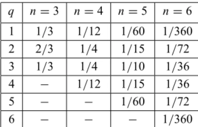
Proposition 5.3. Let n ≥3. For any q∈ {1, . . . ,n}, one has
̺(Uq,n) =
2 n!
n−1 q−1
!
= 2
n(q−1)!(n−q)!. (24)
In particular,
(a) ̺(Uq,n)=̺(Un−q+1,n).
(b) ̺(Uq,n)is minimized at q =1and at q=n.
(c) If n is odd, then̺(Uq,n)is maximized at q =(n+1)/2.
(d) If n is even, then̺(Uq,n)is maximized at q =n/2and at q =(n/2)+1.
Proof. Let X be an n-dimensional Gaussian vector. Membership inUq,n is
conditioned to membership in
Aq =
x ∈Rn:max{x1, . . . ,xq−1,xq+1, . . . ,xn} ≤xq .
The fundamental law of conditional probabilities yields
P[X ∈Uq,n] = P
X ∈Uq,n
X ∈ Aq
PX ∈ Aq
+ PX ∈Uq,n
X ∈/ Aq
| {z }
=0
PX ∈/ Aq
.
Clearly, P[X ∈ Aq] =1/n. On the other hand, stochastic independence of the
components ofX and Corollary 5.2 yield PX ∈Uq,n
X ∈ Aq
= PX1≤. . .≤ Xq−1, Xq+1≥. . .≥ Xn
= PX1≤. . .≤ Xq−1
| {z }
1/(q−1)!
PXq+1≥. . .≥ Xn
| {z }
1/(n−q)!
.
Proposition 5.1 completes the proof of (24). The by-products (a)-(d) are
q n =3 n=4 n=5 n=6 1 1/3 1/12 1/60 1/360 2 2/3 1/4 1/15 1/72 3 1/3 1/4 1/10 1/36
4 − 1/12 1/15 1/36
5 − − 1/60 1/72
6 − − − 1/360
Table 3 – Volumetric moduli of the unimodal conesUq,n.
Proposition 5.1 can also be used for estimating the volumetric modulus of a convex coneK having no structure whatsoever. The basic idea is producing a large sample
X(1),X(2), . . . ,X(N) ≡ (
stochastically independent n-dimensional Gaussian vectors
and counting the number of times that the targetKis being hit. If one introduces the Bernoulli variables
Yi =
(
1 if X(i)
∈ K, 0 if otherwise,
then Proposition 5.1 and the law of large numbers yield the approximation
̺(K)≈2Y1+. . .+YN
N . (25)
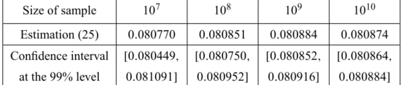
We have tested such a random approximation technique on the cone of Ex-ample 3.4. As shown in Table 4, the size of the random sEx-ample is a key factor for obtaining an acceptable degree of approximation. Confidence intervals at a 99% confidence level are also provided. Of course, sharper confidence in-tervals are obtained if one contents oneself with a confidence level at 95%, as is common in practice.
Table 5 reports on the random estimation technique applied to the Lorentz cone Ln, the Pareto cone Rn+, and the downward monotonic cone Dn. The
estimates for the Pareto cone are consistent with the values predicted by the formula̺(Rn
+) = (1/2)
n−1. Consistency is also observed in the case of the
Size of sample 107 108 109 1010 Estimation (25) 0.080770 0.080851 0.080884 0.080874 Confidence interval [0.080449, [0.080750, [0.080852, [0.080864,
at the 99% level 0.081091] 0.080952] 0.080916] 0.080884]
Table 4 – Random estimation technique for the volumetric modulus of the coneKof Example 3.4.
n=4 n=5 n=6
̺(Ln) 0.181690 0.116117 0.075587
0.181684 0.116119 0.075587 ̺(Rn
+) 0.125000 0.062500 0.031250
0.125000 0.062500 0.031252 ̺(Dn) 0.083333 0.016667 0.002778
0.083335 0.016665 0.002778
Table 5 – Volumetric moduli of the Lorentz cone, the Pareto cone, and the downward monotonic cone. For each dimensionn, one uses a sample of 1010 stochastically independent Gaussian vectors. Exact values are indicated in bold characters.
6 Divide-and-conquer strategy
Sometimes it helpful to decompose a convex coneK as finite union
K = K1∪. . .∪Kℓ, (26)
and then compute the volumetric modulus of each component. Measure dis-jointness of the components can be ensured by assuming a suitable separation property. The rational behind such a divide-and-conquer method is explained in the next proposition.
Proposition 6.1. Let K ∈4(Rn)be decomposed as in(26), where{K1, . . . ,
Kℓ}are elements of4(Rn)satisfying the separation assumption
dim[span(Ki∩Kj)] ≤n−1 for all i 6= j. (27)
Proof. By De Moivre inclusion-exclusion principle for the volume of a finite union, one has
vol(K ∩Bn) = vol ℓ
[
i=1
(Ki ∩Bn)
!
=
ℓ
X
k=1
(−1)k−1 X I⊂{1,...,ℓ} card(I)=k
vol \
i∈I
(Ki ∩Bn)
!
.
The property (27) says that the linear space spanned by each intersectionKi∩Kj
has dimension less thann. Hence,∩i∈I(Ki ∩Bn) has zero volume whenever
card(I)≥2. One gets in this way
vol(K∩Bn)= ℓ
X
i=1
vol(Ki ∩Bn) ,
remaining now to divide on each side by the half-volume ofBn.
Proposition 6.1 is fairly simple as a mathematical result. The two examples below illustrates how such proposition works in practice.
Example 6.2. In the same way as Archimedes approximates a circle by a p -sided polygon, one can approximate the three-dimensional Lorentz cone L3by
a p-faced pyramidal cone
3p =cone
γ (t1), . . . , γ (tp) , (28)
where γ (t) = (1/√2) (cost,sint,1)T and ti = (2i − 1)π/p for all i ∈
{1, . . . ,p}. Suppose that p ≥ 4. How to compute the volumetric modulus of3p? In view of the linear dependence of the generators, neither the numerical
integration method, nor the power series method can be applied in this case. A natural alternative is using a divide-and-conquer strategy: one decomposes (28) as a union of pmeasure-disjoint pieces, namely, Ki =cone{γ (ti), γ (ti+1),e3}.
Heree3 = (0,0,1)T and, by convention, tp+1 = t1. A matter of symmetry
shows that all the components Ki have the same volumetric modulus. Hence,
by applying Proposition 6.1 and the triple product formula (5), one gets
̺(3p)= p̺(K1)=
p
π arctan
sin(2π/p) 3+2√2+cos(2π/p)
Note that limp→∞̺(3p)=1−(
√
2/2)=̺(L3), in consistency with
Proposi-tion 2.1 and Corollary 2.4.
Example 6.3. How to compute the volumetric modulus of a polyhedral convex cone
K =x ∈Rn: hhj,xi ≥0 for all j =1, . . . ,n−1
given by a collection {h1, . . . ,hn−1
}of only n −1 linearly independents unit vectors ofRn? Again, the numerical integration method and the power series
method must be ruled out. We introduce then an additional vectorhnwhose role
is cuttingK into two measure-disjoint pieces:
K1 = {x ∈ K : hhn,xi ≥0},
K2 = {x ∈ K : hhn,xi ≤0}.
The separation property (27) holds becauseK1∩K2is contained in the
hyper-plane with normal vector hn. In the present situation, the cleverest way of defining the missing vectorhnis by solving the linear system
hhj,hni =0 for all j ∈ {1, . . . ,n−1}.
With such a choice ofhn, the componentsK
1andK2have the same volumetric
modulus. By Proposition 6.1, one has̺(K) = 2̺(K1). In order to evaluate ̺(K1), one can use for instance the numerical integration method.
The purpose of Example 6.3 has been preparing the ground for handling a more general situation. The next proposition comes now without surprise.
Proposition 6.4. Consider a polyhedral convex cone
K =x ∈Rn: hhj,xi ≥0 for all j =1, . . . ,r , (29)
where r ≤ n −1and{h1, . . . ,hr}is a collection of linearly independent unit vectors ofRn. Then,
̺(K)=2n−r̺(Kb), (30) whereK is any simplicial reduction of K in the sense thatb
b
with {hr+1, . . . ,hn
} forming an orthonormal basis of the linear subspace [span{h1, . . . ,hr
}]⊥.
Proof. If {hr+1, . . . ,hn
} forms a basis of the orthogonal complement of span{h1, . . . ,hr},then the full collection{hj}nj=1 is linearly independent. Or-thogonality of such basis ensures that the measure-disjoint pieces
Ki =
x ∈ K : hεi,jhj,xi ≥0 for all j =r +1, . . . ,n (31)
have the same volumetric modulus. Each Ki is associated to a vector (εi,r+1, . . . , εi,n) in the lattice {−1,1}n−r. The convex cone Kb is just one of
the 2n−r pieces listed in (31).
Recall that simplicial cone in Rn is a polyhedral convex cone generated by
n linearly independent vectors. This explains the use of the term “simplicial” while referring to Kb. The linearly independent generators {g1, . . . ,gn
} of Kb are obtained by normalizing each column of the matrix H(HTH)−1, where
H = [h1, . . . ,hn]. On the other hand, one uses the term “reduction” becauseKb is strictly contained inK.
Example 6.5. Let Vn be the set of n-dimensional vectors whose
second-order differences are nonnegative, i.e.,
Vn=
x ∈Rn:xj+1+xj−1−2xj ≥0 for all j =2, . . . ,n−1 .
The set Vn is a polyhedral convex cone expressible as intersection of n −2
half-spaces. A simplicial reduction ofVn can be constructed as follows. The
normal vector corresponding to the j-th hyper-space is hj =(√6/6) (0, . . . ,0,1,−2,1,0. . . ,0)T,
where “−2” appears in the j-th coordinate. The scalar√6/6 has been intro-duced just to make sure thatkhjk = 1, although one could dispense with this normalization condition. The vectors
u = (1,1, ...,1)T,
v = (1−n,3−n,5−n, ....,n−3,n−1)T,
are orthogonal among themselves, and also orthogonal to the vectors{h2, . . . ,
hn−1
}. So, one can takeh1
=u/kukandhn
7 Comparing̺with other solidity indices
A solidity index in the axiomatic sense of [15] is a continuous function g:(4(Rn), δ)→Rsuch that
• g(K)=0 if and only ifK is not solid, • g(K)=1 if and only ifK is a half-space, • gis monotonic with respect to set inclusion,
• gis invariant with respect to orthogonal transformations.
As mentioned in Section 2, the volumetric modulus ̺ qualifies as a solidity index. Two other interesting examples of solidity indices are
̺met(K)= inf Q∈4(Rn)
Qnot solid
δ(Q,K) (32)
and
̺frob(K)=
(
radius of the largest ball centered
at a unit vector and contained in K. (33) The “metric” solidity index (32) has been extensively studied in [15, 16, 18]. It has been established in [18, Corollary 2] that
̺met(K)=cos
θmax(K+)
2
, (34)
whereK+stands for the dual cone ofK and
θmax(P)= max
x,y∈P∩Snarccoshx,yi
denotes the maximal angle ofP ∈4(Rn). Concerning the “Frobenius” solidity
index (33), a wide range of applications and relevant material can be found in [6, 8, 9, 13, 14, 15].
Example 7.1. Consider the case of a downward monotonic cone. It has been shown in [14] that
̺frob(Dn)=
s
6
n(n−1)(n+1) ≈
√ 6
On the other hand, by relying on (34) and [12, Proposition 2] one can prove that
̺met(Dn)=cos
1−1
n
π 2
≈ π
2n. (36)
Note that̺(Dn)=2/n!is “much” smaller than both (35) and (36).
Example 7.2. Leta ∈ Sn. For a circular cone with half-aperture angle ϑ ∈
]0, π/2[one obtains
̺frob(Ra,ϑ)=̺met(Ra,ϑ)=sinϑ,
a number which is independent ofn. By constrast, ̺(Ra,ϑ)does depend onn as one can see from Proposition 2.3.
Examples 7.1 and 7.2 will do by way of illustration. The question that we would like to explore now is whether there is some kind of general relationship between̺and the other two solidity indices. Observe that
̺frob(K)≤̺met(K) for allK ∈4(Rn).
This is simply because ̺met is the largest one among all the solidity indices
that are nonexpansive (cf. [15]). The next definition will be useful.
Definition 7.3. Two solidity indicesg1,g2:4(Rn)→Rnare:
i) linearly comparableif there are positive constants a and b, depending possibly onn, such thatag2≤ g1≤bg2.
ii) equivalentif there is an increasing surjectionϕ : [0,1] → [0,1]such that g2=ϕ◦g1.
We start by stating two negative results2.
Proposition 7.4. ̺is neither linearly comparable to̺frobnor to̺met. 2Note added in proof: We have been able, however, to prove that̺
≤̺met. This result will
Proof. We prove the following claim: there is no positive constantasuch that a̺frob≤̺. To do this, we show that
inf
K∈4(Rn)
Ksolid
̺(K) ̺frob(K) =
0.
Let us evaluate the quotient̺/̺frobon a circular coneRa,ϑ and then letϑgo to zero. By applying L’Hôpital’s rule, one gets
lim ϑ→0+
̺(Ra,ϑ) ̺frob(Ra,ϑ) =
lim ϑ→0+
Fn(ϑ )
sinϑ =ϑlim→0+ κ−1
n (sinϑ)n−2
cosϑ = 0.
The case of̺metis treated in exactly the same way.
Proposition 7.5. ̺is neither equivalent to̺frobnor to̺met.
Proof. The function Fn introduced in Proposition 2.3 is a bijection from
[0, π/2] to [0,1]. Let ϑn be the unique solution to the nonlinear equation
Fn(ϑ)=(1/2)n−1.Then̺(Ra,ϑn)=̺(R
n
+), regardless of the choice ofa∈Sn.
But, on the other hand,
̺met(Ra,ϑn) = sinϑn 6=
p
1/2 = ̺met(Rn+).
This rules out the possibility of finding an increasing surjective function ϕ :
[0,1] → [0,1]such that̺ =ϕ◦̺met. In short,̺and̺met are not equivalent.
One can also check that
̺frob(Ra,ϑn) = sinϑn 6=
p
1/n = ̺frob(Rn+).
Hence,̺is not equivalent to̺frobeither.
Despite the negative results stated in Propositions 7.4 and 7.5, there is a link between̺ and̺frob after all. However, such a link is nonlinear in nature and
quite sophisticated.
Theorem 7.6. For all K ∈4(Rn)one has
1 κn
Z ̺frob(K)
0
tn−2
√
as well as
1− 1 κn
Z ̺frob(K+)
0
hp
1−t2in−3dt ≥ ̺(K). (38)
Both inequalities become equalities if and only if K is a circular cone.
Proof. A natural idea that comes to mind is estimating ̺(K) by using the inner and outer circular approximations
Kinn ≡ largest circular cone contained inK,
Kout ≡ smallest circular cone containingK.
Letθinn(K)andθout(K)denote the half-aperture angles ofKinnandKout,
respec-tively. As a consequence of Proposition 2.3, one gets
1 κn
Z θinn(K)
0
(sint)n−2dt ≤ ρ(K) ≤ 1 κn
Z θout(K)
0
(sint)n−2dt. (39) Let us work out both sides of the above sandwich. It can be shown that
sin [θinn(K)] = ̺frob(K), (40)
cos [θout(K)] = ̺frob(K+). (41)
Formula (41) is obtained by combining [17, Theorem 7] and [15, Proposi-tion 6.3]. Formula (40) is obtained from (41) by using duality arguments. Hence,
1 κn
Z θinn(K)
0
(sint)n−2dt = Gn(̺frob(K)),
1 κn
Z θout(K)
0
(sint)n−2dt = Hn(̺frob(K+))
withGn,Hn: [0,1] → [0,1]given respectively by
Gn(r)=Fn(arcsinr) =
1 κn
Z r
0
tn−2 √
1−t2dt,
Hn(r)= Fn(arccosr) = 1−
1 κn
Z r
0
hp
1−t2in−3dt.
Corollary 7.7. For all K ∈4(Rn)one has
1 (n−1)κn
̺frob(K)
n−1
≤ ̺(K). (42)
Proof. It is enough to observe that
tn−2
√
1−t2 ≥ t n−2
.
Thus, the inequality (42) is a weakening of (37).
We stated Corollary 7.7 just to indicate that̺can be minorized by a positive multiple of the power ̺frob(∙)
n−1
. Recall that ̺ cannot be minorized by a positive multiple of̺frobitself.
8 By way of conclusion
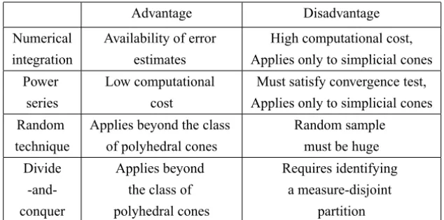
In this work we have discussed several methods for computing the volumetric modulus of a convex cone. Table 6 gives a general overview of the advantages and disadvantages of each method. The details can be consulted in the corre-sponding section.
Advantage Disadvantage
Numerical Availability of error High computational cost, integration estimates Applies only to simplicial cones
Power Low computational Must satisfy convergence test,
series cost Applies only to simplicial cones
Random Applies beyond the class Random sample
technique of polyhedral cones must be huge
Divide Applies beyond Requires identifying
-and- the class of a measure-disjoint
conquer polyhedral cones partition
Table 6 – Methods for computing volumetric moduli.
The next example concerns a nasty convex cone arising in Moving Average Estimation (cf. [1, 3]).
Example 8.1. Let d ≥ 2. One says that x = (x0, . . . ,xd) ∈ Rd+1 is an
autocorrelation vectorif there existsz =(z0, . . . ,zd)∈Rd+1such that
xk = d−k
X
i=0
zizi+k for all k ∈ {0,1, . . . ,d}.
LetCd
+1denote the set of all autocorrelation vectors inRd+1. It is known that
Cd
+1is representable in the form
Cd
+1=
(
x ∈Rd+1:x0+2 d
X
k=1
xkcos(kw)≥0, ∀w∈ [0, π]
)
. (43)
By using this frequency-domain characterization, it is not difficult to show that
Cd
+1is a solid pointed closed convex cone.
The convex cone of Example 8.1 is not polyhedral. Hence, the numerical integration method and the power series method must be ruled out. On the other hand, it is not clear how to partitionCd+1 in terms of measure-disjoint convex
cones with easily computable volumetric moduli. We are left with the random technique as only option. However, checking if a given vector belongs toCd
+1
is not a trivial matter, and the cost of this operation must be multiplied by the size of the random sample. Note that the right-hand side of (43) is a set defined by infinitely many contraints.
For dealing with a desperate situation like this, there are at least two possibil-ities. The first option is estimating̺(K)by using the sandwich (39). In fact, one does not need actually to compute the exact values ofθinn(K)andθout(K).
Given the monotonicity ofϑ 7→R0ϑ(sint)n−2dt, it is perfectly acceptable to use a lower bound forθinn(K)and a upper bound forθout(K). Let us see how this
principle works in the case of the cone of autocorrelation vectors.
Corollary 8.2. For d≥2, one has
1 κd+1
Z αd
0
(sint)d−1dt ≤ ̺(Cd
+1) ≤
1 κd+1
Z βd
0
with
αd = arcsin
h
1/√1+4di, βd = arccos
inf{x0:x ∈Cd+1,kxk =1}
.
Proof. Writex =(x0, ξ )withx0∈Randξ ∈Rd. For allw∈ [0, π], one has
x0+2 d
X
k=1
xkcos(kw) ≥ x0−2kξk
" d X
k=1
cos2(kw)
#1/2
≥ x0−2kξk
√ d.
By using these inequalities, one can show that the circular cone with axisa =
(1,0, . . . ,0)∈Sd+1and half-aperture angleαdis contained inCd
+1. Hence,αd
is a lower estimate forθinn(Cd+1). On the other hand,
cosθout(Cd+1)
= sup
kyk=1
inf
x∈Cd +1
kxk=1
hy,xi
≥ inf{x0:x ∈Cd+1,kxk =1},
i.e.,βdis a upper estimate forθout(Cd+1).
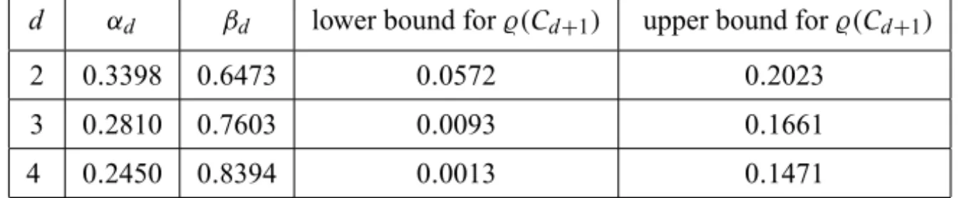
Table 7 displays the numerical values of the bounds (44) for the casesd =2,
d =3, andd =4. The bounds for̺(Cd+1)could be sharpened by using the exact
values ofθinn(Cd+1)andθout(Cd+1). However, one should not be over optimistic
becauseCd
+1 is far from being a circular cone. The situation gets even worse
whendincreases. We must say things as they are: the estimates given in Table 7 are very disappointing. The method of inner and outer approximation by circular cones is ill suited in the case of the cone of autocorrelation vectors.
d αd βd lower bound for̺(Cd+1) upper bound for̺(Cd+1)
2 0.3398 0.6473 0.0572 0.2023
3 0.2810 0.7603 0.0093 0.1661
4 0.2450 0.8394 0.0013 0.1471
Table 7 – Bounding̺(Cd
+1) by using inner and outer circular approximations. Figures are
A second and much better possibility for consideration is using an outer poly-hedral approximation
C
d+1=
(
x ∈Rd+1:x0+2 d
X
k=1
xkcos(kw)≥0, ∀w∈
)
(45)
of the coneCd
+1. Here= {w0, . . . , wN}stands for a finite collection of points
in[0, π]. One gets in this way the upper estimate
̺ Cd
+1
≤̺ C
d+1
.
In Table 8 one considers a regular partition of[0, π], i.e.,wi =iπ/N for all
i ∈ {0,1, . . . ,N}. This implies that (45) is a polyhedral convex cone defined by card()= N +1 contraints. The volumetric modulus ofC
d+1is estimated
by using the random technique. For obtaining each entry in Table 8, one works with a sample of 108stochastically independent Gaussian vectors.
d N =10 N =20 N=50 N =100
2 0.1091 0.1083 0.1080 0.1079
3 0.0387 0.0359 0.0357 0.0356 4 0.0137 0.0129 0.0126 0.0126
Table 8 – Volumetric modulus ofC
d+1. Figures are rounded to four decimals.
As far as the first four decimals are concerned, the term ̺(C
d+1) does not
change significatively if the mesh parameter N goes beyond 100. Observe that the upper bounds for̺(Cd
+1)provided by the last column of Table 8 are much
sharper than the corresponding upper bounds given in Table 7.
Remark 8.3. Ifis a regular mesh whose cardinality goes to∞, thenC
d+1
converges toCd
+1 with respect to the metricδ. The proof of this fact is long
and tedious, so it will not be presented here. Such a convergence result indicates that̺(C
d+1)can be made arbitrarily close to ̺(Cd+1) by suitably refining the
REFERENCES
[1] B. Alkire and L. Vandenberghe,Convex optimization problems involving finite
autocorrela-tion sequences. Math. Program.,93(2002), 331–359.
[2] V. Boyarshinov and M. Magdon-Ismail,Linear time isotonic and unimodal regression in the
L1and L∞norms. J. Discrete Algorithms,4(2006), 676–691.
[3] B. Dumitrescu, P. Stoica and I. T˘abu¸s, On the parameterization of positive real sequences
and MA parameter estimation. IEEE Trans. Signal Process.,49(2001), 2630–2639.
[4] R.L. Dykstra and J.H. Lemke, Duality of I projections and maximum likelihood estimation
for log-linear models under cone constraints. J. Amer. Statist. Assoc.,83(1988), 546–554.
[5] M.L. Eaton and T. Kariya, Robust tests for spherical symmetry. Ann. Statist.,5(1977), 206–215.
[6] M. Epelman and R.M. Freund, A new condition measure, preconditioners, and relations
between different measures of conditioning for conic linear systems. SIAM J. Optim.,
12(2002), 627–655.
[7] F. Eriksson,On the measure of solid angles. Math. Mag.,63(1990), 184–187.
[8] R.M. Freund, On the primal-dual geometry of level sets in linear and conic optimization. SIAM J. Optim.,13(2003), 1004–1013.
[9] R.M. Freund and J.R. Vera, Condition-based complexity of convex optimization in conic
linear form via the ellipsoid algorithm. SIAM J. Optim.,10(1999), 155–176.
[10] M.P.C. Fossorier and A. Valembois, Sphere-packing bounds revisited for moderate block
lengths. IEEE Trans. Inform. Theory,50(2004), 2998–3014.
[11] W. Gao and N.Z. Shi, I -projection onto isotonic cones and its applications to maximum
likelihood estimation for log-linear models. Ann. Inst. Statist. Math.,55(2003), 251–263.
[12] D. Gourion and A. Seeger, Critical angles in polyhedral convex cones: numerical and
statistical considerations. Math. Program.,123(2010), 173–198.
[13] R. Henrion and A. Seeger, On properties of different notions of centers for convex cone. Set-Valued Anal.,18(2010), 205–231.
[14] R. Henrion and A. Seeger, Inradius and circumradius of various convex cones arising in
applications. Set-Valued Anal., to appear.
[15] A. Iusem and A. Seeger, Axiomatization of the index of pointedness for closed convex
cones. Comput. Applied Math.,24(2005), 245–283.
[16] A. Iusem and A. Seeger, Measuring the degree of pointedness of a closed convex cone: a
metric approach. Math. Nachr.,279(2006), 599–618.
[17] A. Iusem and A. Seeger, Normality and modulability indices. Part I: convex cones in
[18] A. Iusem and A. Seeger,Antipodality in convex cones and distance to unpointedness. Appl. Math. Letters,21(2008), 1018–1023.
[19] A. Iusem and A. Seeger, Antipodal pairs, critical pairs, and Nash angular equilibria in
convex cones. Optimiz. Meth. Software,23(2008), 73–93.
[20] J.M. Ribando,Measuring solid angles beyond dimension three. Discrete Comput. Geom.,
36(2006), 479–487.
[21] A. van Oosterom and J. Strackee,The solid angle of a plane triangle. IEEE Trans. Biomed. Eng.,30(1983), 125–126.
[22] A. Seeger and M. Torki, Local minima of quadratic forms on convex cones. J. Global Optim.,44(2009), 1–28.
[23] C. Shannon, Probability of error for optimal codes in a Gaussian channel. Bell System Tech. J.,38(1959), 611–656.