Interactive graphics tool for the calculation and
serviceability limit state stress check of bonded
post-tensioned concrete beams according to brazilian codes
via Autodesk Robot Structural Analysis Professional
®
Ferramenta gráico-interativa de cálculo e veriicação
de tensões no estado limite de serviço de vigas
protendidas com pós-tração aderente para a norma
brasileira através do Autodesk Robot Structural
Analysis Professional
®
Abstract
Resumo
This work presents an interactive graphics computational tool for the veriication of prestressed concrete beams with post-tensioned bonded ten-dons to the serviceability limit state (SLS) stress check according to the Brazilian code NBR 6118:2014. The tool is an add-in for Autodesk Robot Structural Analysis Professional®, which serves as a structural modeling platform.
With data supplied by the user through a graphics user interface, the program here developed calculates all relevant prestress losses that occur throughout the structure’s life-cycle, along with the prestress’ equivalent loads during this period. The traditional calculation methods, obtained in the NBR 6118, are presented along with the modiications which had to be implemented in order to allow for incremental loss calculations. Usage examples and results are presented, validating the adopted methodology.
At the end of the software’s calculation, the user receives two outputs: the prestress’ equivalent loads in the Robot model and an Excel spread-sheet. The spreadsheet contains the resultant stresses in the beam and warns whether these are greater than the permissible stresses in the SLS stress check. The loads may then be used in other calculations, such as shear reinforcement.
Keywords: prestressed concrete beams, ABNT NBR 6118, serviceability limit state stress check, Autodesk Robot Structural Analysis Professional®.
Este trabalho apresenta o desenvolvimento de uma ferramenta computacional gráico-interativa para a veriicação de vigas de concreto protendi-do com pós-tração aderente ao estaprotendi-do limite de serviço (ELS), de acorprotendi-do com a norma brasileira NBR 6118:2014. A ferramenta é um add-in para o Autodesk Robot Structural Analysis Professional®, que serve como plataforma de modelagem estrutural.
A partir de dados fornecidos pelo usuário através de uma interface gráica, o programa desenvolvido calcula todas as perdas de protensão que ocorrem ao longo da vida-útil da estrutura, assim como os carregamentos equivalentes à protensão durante este período. O trabalho apresenta os métodos de cálculo tradicionais, obtidos da NBR 6118, e as modicações que tiveram que ser feitas para permitir um cálculo incremental. Exemplos de utilização do programa também são apresentados, validando a metodologia adotada.
Ao im do cálculo o usuário recebe duas saídas: os carregamentos equivalentes da protensão ao longo da vida-útil da estrutura no modelo do Robot e uma planilha Excel. A planilha contém os esforços e as tensões atuantes na viga ao longo de sua vida-útil e informa se estes valores ultrapassam os limites estabelecidos para o ELS. Os carregamentos podem ser utilizados para demais carregamentos, tal como no dimensiona-mento ao esforço cortante.
Palavras-chave: Vigas de concreto protendido, ABNT NBR 6118, Estado limite de serviço (ELS), Autodesk Robot Structural Analysis Professional®.
P. K. K. NACHT a
L. F. MARTHA a
1. Introduction
The Building Information Modeling (BIM) philosophy is revolution-izing structural engineering. The fundamental concept is to bring all the information from the disparate disciplines into a single data-base. One then has a single structural model which incorporates all the structure’s life-cycle information: architectural, structural, hydraulic, electric, mechanical, as-built, and maintenance projects. Prestressed concrete structures, however, tend to be modeled separately in specialized software which does not attempt to follow the BIM philosophy.
To aid in the uniication of prestressed structural models with BIM, this work presents a computational tool for the serviceability limit state stress check of bonded post-tensioned concrete beams ac-cording to Brazilian codes via Autodesk Robot Structural Analy-sis Professional®, henceforth referred to as Robot. This software,
named Prestress, is an add-in for Robot, leveraging its structural modeling capabilities to obtain the loads and stresses arising from the prestress.
Robot was chosen as the platform for Prestress because it is part
of the Autodesk environment. BIM does not require that a single company’s package be adopted, but open-source databases, com-monly represented by IFC iles, cannot as of yet contain all of the “intelligence” of a model [1]. For this reason, though it is not strictly necessary, adopting a company’s closed environment simpliies the implementation of the BIM philosophy for now. With Robot as a platform, Prestress can now unify the prestressing calculations
to those of the global structure. Though not yet implemented, Pre-stress can still be extended to add the prestressing to an Autodesk
Revit 4D model to check for possible interferences and inclusion in the structure’s life-cycle analysis.
From a structural model created within Robot and prestressing
data given by the user, prestress losses are calculated, isostatic bending moments are obtained and equivalent loads are applied. The program’s calculations are boundary-condition-agnostic, suc-cessfully dealing with isostatic and statically indeterminate beams. The effects of the boundary conditions are considered by Robot
and incorporated in Prestress. Once the (possibly statically
in-determinate) stresses are obtained, the software then performs a serviceability limit state stress check on the beam and generates an .xlsx ile containing the results.
A limitation of Prestress at present is that it cannot correctly
cal-culate structures which are built in stages. While Robot has what it calls “phase structures”, its API does not implement any method by which external programs (such as Prestress) can retrieve
infor-mation regarding the different construction phases [2]. It is there-fore impossible for Prestress to accurately calculate segmental
bridges or prefabricated beams with cast-in-place decks which are usually considered to work with the beam for live-loads.
There are at present already multitudes of software in the mar-ket which aid the engineer in the design of prestressed concrete structures. midas Civil®, SAP 2000®, ADAPT-ABI®, ADAPT-PT/
RC®, RAPT® and Nemetschek Scia® are but a few of the available
options. All of these are evidently far more advanced and robust
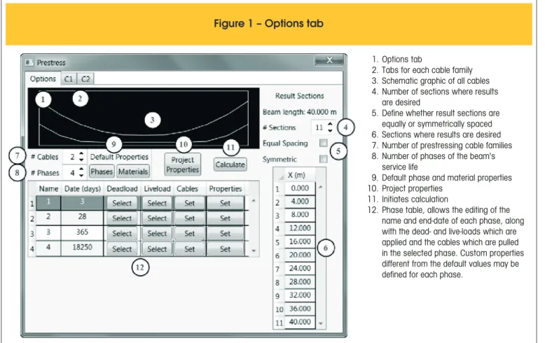
Figure 1 – Options tab
01. Options tab
02. Tabs for each cable family 03. Schematic graphic of all cables 04. Number of sections where results
are desired
05. Define whether result sections are equally or symmetrically spaced 06. Sections where results are desired 07. Number of prestressing cable families 08. Number of phases of the beam's
service life
09. Default phase and material properties 10. Project properties
11. Initiates calculation
than the software here developed. However, of the above only
ADAPT-PT/RC® currently performs the calculations and
service-ability checks according to the Brazilian codes, but it is a 2D-only platform. There are other programs, such as those developed by Bortone [3] and Lazzari et al. [4], which fall into the same category.
Prestress is unique in that it follows the Brazilian codes and
al-lows the user to work in a 3D space. Compared to the works of Bortone and Lazzari et al., it also has the advantage of not being a stand-alone program. This means the engineer need not create two structural models: one to calculate the prestressed element and another to obtain the behavior of the rest of the structure. Having the prestressing loads within the global structural model also allows the user to observe the effect of the prestress in the entire structure. The following sections will present the procedures adopted by the software and two examples. One example is that of an isostatic beam, while the other is of a statically indeterminate structure. Each example presents the information relevant for prestressing and the ile containing the results.
2. Procedure
2.1 Input
The Prestress software requires that the user already have a
complete structural model deined in Robot, including constraints
and load cases. It is essential that the beam be allowed to deform
must be taken in the deinition of the constraints. For instance, if a beam’s two extremities have constraints which do not allow the beam to be compressed, a large part of the prestress will be lost. The user then selects the beam to be prestressed, which may be composed of one or more bar segments. Via a graphical user inter-face, the engineer may input the requisite prestressing data. This includes the number of cables, each cable’s longitudinal layout, section area, pull stress, and relevant prestress loss coeficients, as well as material properties for both concrete and steel and the desired level of prestress: limited or complete prestress. Partial prestress, which permits the concrete to crack in tension, is not al-lowed. The units adopted by Prestress are taken directly from the Robot model, so as to allow the user to work with the unit system
(s)he has previously deined.
Another key piece of data the user must present is the different phases of a structure’s lifecycle. The suggested minimum number of such phases is four [5], representing: the age of concrete at pre-stressing; when loads other than self-weight and prestress are ap-plied; one year; and the end of the structure’s service life. The user, however, is free to alter both the number and dates of phases. Each phase is deined by the concretes age at the end of the phase, the dead and live loads that are applied and the cables that are jacked on that phase, along with representative values of temperature and humidity for that phase. Should the prestressing operation occur in multiple stages, this should be represented in the user’s input, pref-erably by including additional phases. Figures [1] and [2] show the
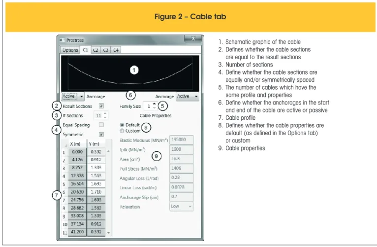
Figure 2 – Cable tab
1. Schematic graphic of the cable 2. Defines whether the cable sections are equal to the result sections 3. Number of sections
4. Define whether the cable sections are equally and/or symmetrically spaced 5. The number of cables which have the same profile and properties
6. Define whether the anchorages in the start and end of the cable are active or passive 7. Cable profile
8. Defines whether the cable properties are default (as defined in the Options tab) or custom
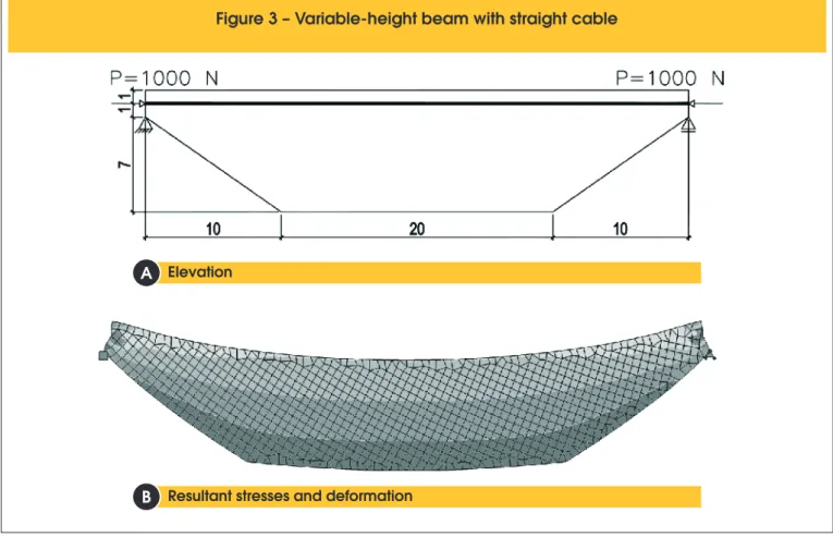
Figure 3 – Variable-height beam with straight cable
Elevation
A
Resultant stresses and deformation
B
Figure 4 – Variable-height beam with variable cable
Elevation
A
Resultant stresses and deformation
With this data Prestress then calculates all relevant prestressing losses: friction, anchorage slippage, concrete elastic deformation, creep and shrinkage, and steel relaxation.
2.2 Equivalent loads
A curved cable under tension tends to straighten, but this is im-peded by the concrete and its self-weight, so the cable applies a distributed force along the beam’s span. The standard method of deining an equivalent load to simulate this force was presented by Lin [6]. For a beam with a parabolic cable of length L, pull-force P and maximum delection e, the equivalent distributed load is given by Equation [1].
(1)
This method, however, is not generic since it requires a beam of constant section [7]. Figures [3], [4] and [5] present three different variable beams. The first presents a beam of vari-able height, prestressed with a straight tendon. Though the tendon has no deflection, the eccentricity of the cable to the beam’s centroid is variable, leading to a flexural stress-state in the beam. The second presents a beam with variable height but with a polygonal cable which always follows the beam’s centroid. Though the cable has a deflection, in this case the beam’s stress-state is that of pure compression. The third case presents a beam with a sudden change of section. It is clear that where the cable is aligned with the centroid, the beam is under pure compression, but where the cable is offset from the centroid, the beam presents a bending moment. It is
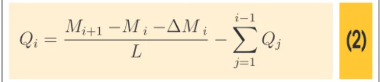
there-fore necessary to adopt a more generic function for equiva-lent loads. The adopted solution applies concentrated loads according to Equation [2] at every section i where the cable’s layout was defined, where Mi and Mi+1 are the isostatic pre-stressing bending moments at the current section and the fol-lowing one, respectively, and ΔM is the difference between the bending moment immediately to the right and left of the cur-rent section and is therefore only non-zero if there is a cross-section discontinuity at point i. If such a discontinuity occurs, a concentrated moment equal to ΔM must also be applied.
(2)
This method generates a polygonal approximation of the beam’s prestressing bending moment diagram, regardless of the boundary conditions. If the structure is statically indeter-minate, then the boundary conditions will naturally generate the correct diagram. This equivalent load method also satis-fies the condition of being self-balanced, generating no reac-tions on supports in isostatic structures. Prestress losses are also trivially considered, since the values of Mi and Mi+1 are naturally calculated after all relevant losses. Figure [6] shows an example of a beam without cross-section discontinuities (therefore ΔM is always null) under a constant distributed load and the linear approximation via Equation [2]. The errors here are of approximately ±1%, but this is evidently affected by the number of points where concentrated loads are defined. The equivalent loads of each phase of the structure’s service life are left in the model after Prestress is complete, allowing the user to make use of these loads if so desired.
Figure 5 – Beam with section discontinuity and a straight cable
Elevation
A
Resultant stresses and deformation
2.3 Prestress losses
A prestressed cable is jacked up to a speciied stress. This stress, however, is not constant along the cable’s length, nor is it constant in time. The losses can be simply bundled into two groups: imme-diate and progressive losses. The immeimme-diate losses, as the name would imply, happen at the act of jacking. These are losses due to: friction between the cable and its duct; anchorage slippage; and the elastic deformation of the concrete. The progressive losses are time-dependent, ever-approaching an asymptotic value at the end of the beam’s service-life. These are the losses due to steel relax-ation and concrete creep and shrinkage. The methods adopted by
Prestress are summarized below.
Friction losses are calculated according to item 9.6.3.3.2.2 of the NBR 6118:2014 [8], which is itself simply the traditional equation for such losses, seen in Equation [3], where P0 is the pull force;
µ, the angular friction coeficient; α(x), the total absolute angular variation from the anchorage until point x; and k, the linear friction coeficient.
(3)
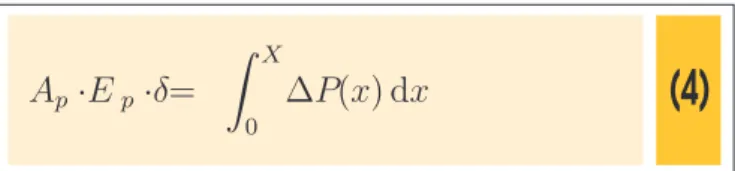
Anchorage slippage losses are calculated by solving Equation [4], where A p is the cable’s cross-section’s area; Ep, the cable’s modu-lus of elasticity; δ, the anchorage’s slip length; ΔP(x), the loss of prestress due to anchorage slippage until point x; and X is the point where these losses end. Prestress adopts the cable’s stress
dia-gram after friction losses and inds X by incrementally calculating the area between this diagram and its version mirrored over P(X).
Figure 6 – Beam under distributed and equivalent loads
Beam under constant distributed load
Approximation of distributed load
A
C
Statically indeterminate and isostatic bending moment diagrams under distributed load
Approximate isostatic and statically indeterminate bending moment diagrams
B
(4)
Losses due to the elastic deformation of concrete from prestress-ing and dead loads are also considered. The stresses due to dead loads and equivalent prestressing loads are calculated by Robot
and Equation [5] is applied, where Δσp is the change of stress in the steel; Δσc, in the concrete; and αp is equal to the ratio of the steel and concrete moduli of elasticity.
(5)
Prestress currently only calculates post-tensioned bonded cables.
Such cables only suffer elastic deformation losses due to the pre-stressing of subsequent cables, but not due to their own jacking. If cables are pulled at different dates, then the effect of the jacking of the latter cables will only be computed at that later date. This allows the software to consider the effect of the differed losses (discussed below) on the former cables prior to the inluence of the elastic deformation losses.
The treatment of the progressive losses is more complex. These losses are interdependent, with the result of one altering the result of the other and visa-versa. The methods adopted by Prestress are those present in Annex A of the NBR 6118 [8]. However, they do not allow for the consideration of this interdependence and therefore had to be slightly modiied. Below are described the methods used by the software. When calculating each differed loss for a phase i the program assumes the stresses in phase i-1 are constant. With a suficient number of phases (at least four, as described in Section [2.1]), this allows for an approximation of the true results [5].
Creep losses are calculated by the traditional method of consider-ing a factor φ which represents the deformation increment over time, as seen in Equation [6]:
(6)
Item A.2.2.3 of the NBR 6118 [8] considers φ as the sum of three parts: φa, which represents the quick, plastic deformation which
occurs in the irst 24 hours; φf, the slow, plastic deformation; and φd, the slow, elastic deformation.
φa is calculated by Prestress precisely as in the Brazilian code
according to Equation [7], where β1 is the fraction of the concretes
28-day strength present on t0, the moment the load is applied. The code actually deines the boundaries differently, with the irst case being used for concretes with a compressive strength between 20 and 45MPa, and the second for concretes between 50 and 90MPa. Those used here are equivalent, but also allow for concretes with strengths between 45 and 50MPa. Conservatively, such concretes would fall under the second case. Since this portion of the con-cretes creep occurs in the irst 24 hours, it is only considered in the irst phase after a load is applied.
(7)
φf is calculated in a form almost identical as that given in the code,
as shown in Equation [8], where φf∞ is the asymptote of φf and βf is a time function for such losses. The only difference between this function and the one in the NBR 6118 [8] is that instead of being restricted to t0, the moment the load is applied, it allows the creep increment to be found between any two moments in time. This
Figure 7 – Incremental prestressing loss due to slow, plastic concrete creep. With the increase in
humidity over time the final loss is reduced. To disconsider the humidity's
allows the creep from a load applied at t0 to be computed from t0 to t1 and from t1 to t2… all the way to tn, which deines the end of the structure’s life-cycle. Both φf∞ and βf are functions of the humidity in the air, which means that calculating different phases with vary-ing humidity leads to a different result than if an average value were considered. Figure [7], for instance, demonstrates a ictitious example of a beam in an environment with ever-increasing humid-ity. Notice how the inal result considering only the humidity of the last phase (which represents 49 of the beam’s 50-year service life) leads to a result which is 25% lower than if the varying humidity in the irst year is considered.
(8)
φd is the portion which is most modiied. For the irst increment of time its value is obtained via Equation [9], precisely as deined in
the Brazilian code [8]. For every other increment of time, however, Equation [10] must be used. This occurs due to the peculiar behav-ior of the code’s method, which implies in a non-zero φd for t1 ≈ t0.
(9)
(10)
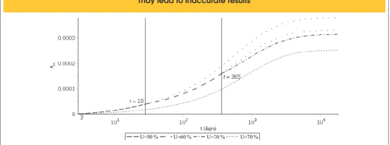
The implementation of prestressing losses due to concrete shrink-age does not require any modiications to the method present in the NBR 6118 [8], seen in Equation [11], where εcs∞ is the maximum value and βs is a time function. Given the deformation increment
Figure 8 – Incremental prestressing loss due to concrete shrinkage. With the increase in humidity
over time the final loss is reduced. To disconsider the humidity's variation over time, however,
may lead to inaccurate results
between two moments, Prestress then needs only to multiply this
value by the steel’s modulus of elasticity to obtain the relevant loss of stress. Figure [8] shows the shrinkage losses over time for a structure in an increasingly humid environment.
(11)
There is, however, one note that must be made in regards to shrinkage losses and that is that the actual value of shrinkage de-formation is a function of a beam’s boundary conditions. The beam segment of a plane frame, for instance, will suffer less shrinkage deformation than a simply supported beam due to the stiffness of
the pillars. Such effects are not considered by the software, which assumes for these losses that the beam has no restrictions to axial deformations. This is a conservative assumption which leads to greater prestressing losses.
Steel relaxation losses are calculated based on item 9.6.3.4.5 of the NBR 6118 [8]. The method, however, had to be modiied some-what to allow for an incremental method as shown in Equation [11], where ψi is the relaxation that occurs between ti and ti-1; ψ1000,i-1, the relaxation coeficient for 1000 hours, obtained in the code’s Table 8.4, considering the cable stress at moment t i-1; and t0, the mo-ment the cable was pulled. Since ψ1000 is a function of steel stress,
which is altered by the other progressive losses, the value of ψ1000 is in fact variable in time. Figure [9] shows a ictitious example of a cable where the value of ψ1000 is progressively reduced, simulating the effect of the other differed losses.
(12)
After calculating each of these losses for every phase of a beam’s service life, Prestress can then apply equivalent loads which
simu-late the prestress. With these equivalent loads in combination with the live and dead loads along the structure’s service life, the soft-ware can then perform the serviceability limit state stress check.
2.4 Serviceability limit state stress check
A prestressed structure must be checked against two limit states: ultimate and serviceability. The ultimate limit state (ULS) certiies that the structure will not collapse when under load. The service-ability limit state (SLS) checks that, if ULS is also satisied, the structure will be adequate for use. A beam which withstands a load but does so with excessive cracking or delection will not give its users peace of mind and may forbid the use of sensitive machin-ery. Both limit states are equally important, but only SLS, which is usually the critical veriication [9], is checked by Prestress. The
user must therefore perform ULS checks by some other means. The Brazilian code deines three levels of live loads, each of which is given a coeficient: rare (ψ0), frequent (ψ1), and almost-perma-nent (ψ2). For a nominal live load Q, the frequent load is therefore
equal to ψ1Q, for example. The values of the coeficients can be
found in Table 11.2 of NBR 6118 [8] or Table 6 of NBR 8681 [10]. Table 13.4 of NBR 6118 [8] states that depending on the environ-mental conditions (CAA, as deined in Table 6.1 of the code), differ-ent stresses are permissible:
n If the environmental conditions are deined as CAA I or II, con-crete cracking is permitted with a speciied maximum nominal crack width (wk,max = 0,2mm) considering frequent loading. This is deined as partial prestress;
n For CAA III or IV, stresses must be checked in two conditions: there must be no tensile stresses in the concrete under almost-permanent loads (ELS-D) and tensile stresses below the con-cretes tensile strength in lexure (fct,f, as deined in item 8.2.5 of NBR 6118) are permissible under frequent loads (ELS-F). This is deined as limited prestress;
n Though never obligatory for post-tensioned structures, there is also a stricter check which only allows tensile stresses below the concretes tensile strength under rare loads (ELS-F) and forbids tensile stresses under frequent loads (ELS-D). This is deined as complete prestress.
Another SLS check is for excessive compression in the concrete (ELS-CE) as per item 17.2.4.3.2.a) of the NBR 6118 [8]. Here the compression must not be greater than 70% of the concretes strength fckj on the date in question, considering a factor of 1.1 on the prestressing loads. Prestress
performs SLS checks under either limited or complete prestress. Item 9.6.1.3 of the NBR 6118 [8] states that the nominal prestress can be considered equal to the value obtained after all required
losses as calculated in Section [2.3], unless the losses are greater than 35% of the initial jacking force. In such a case, the nominal prestress must be considered as ±5% the calculated value. Re-gardless of the magnitude of the losses, Prestress always
consid-ers this variation of the nominal prestress force.
The stress and SLS-check results for the top and bottom ibers of each section are saved in an .xlsx ile, examples of which can be seen in Section [3].
3. Examples
3.1 Santa Isabel Viaduct
The Santa Isabel Viaduct [11] is an isostatic structure which
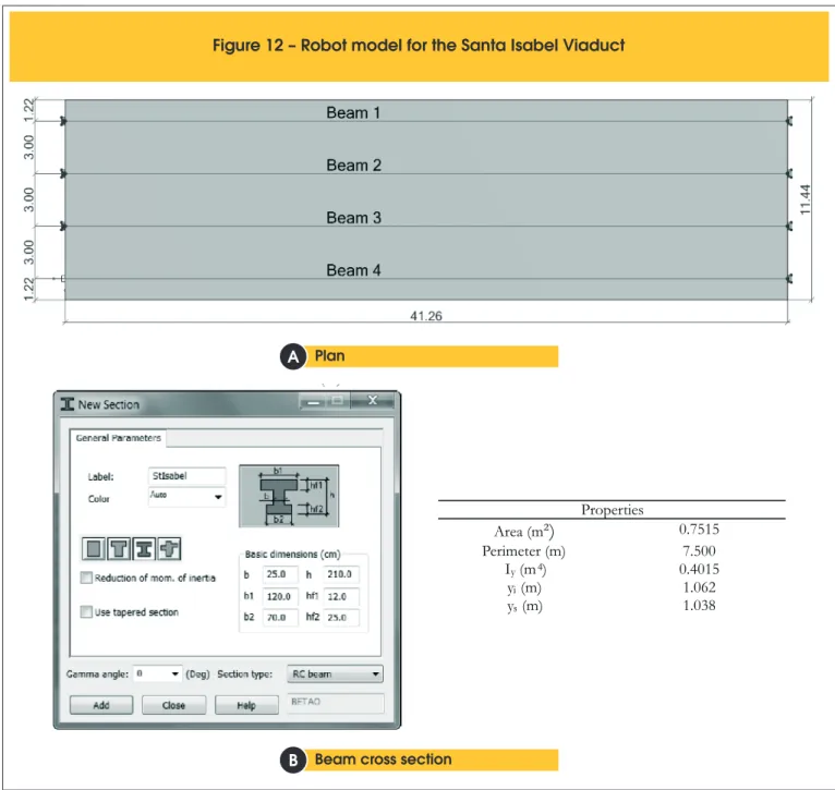
pres-ents a single 41,26m span. The cross-section is composed of four prefabricated beams supporting a 20cm-thick cast-in-place deck. The beams are placed on neoprene bearing pads which allow them to deform in all directions. Figures [10] and [11] and Table [1] present all the relevant information for the prestressing of the beams. The Robot model adopted is shown in Figure [12]. As stated in
Sec-tion [2.1], it is important to observe the boundary condiSec-tions. Since the beams are supported by neoprene pads which allow for both rotation and displacement of the beams, the model was created with all but one of the supports resisting only vertical displacements. A single sup-port is given additional constraints in order to create a stable model. Also note the difference in cross-section properties between the mod-el and the information given in Table [1] due to the simpliication of the section. Since Prestress will adopt the section given in the model,
Figure 12 – Robot model for the Santa Isabel Viaduct
Plan
A
Beam cross section
B
Properties
Area (m
²)
0.7515
Perimeter (m)
7.500
I
y(m
4)
0.4015
y
i(m)
1.062
the results will not be the same as if the true cross-section were used. A more precise representation could have been used via the custom “Section Deinition” option available in Robot.
The fact that it is impossible for any add-in to consider structures built with construction phases means that the model had to suffer some simpliications. The cross-beams at the supports and mid-span were not considered in the model (they are replaced by con-centrated loads on the beams) and the slab is deined as a “clad-ding”, which serves only to distribute loads and does not add to the structure’s stiffness. These simpliications are necessary since the beams are in fact prestressed prior to being hoisted and therefore the entire prestressing load is resisted by the isolated beam. If the cross-beams and the slab added to the stiffness of the model, they would absorb signiicant portions of the prestress load from the beam, leading to imprecise results.
The dead loads are divided into two parts: the beams’ self-weight and that of the slab, pavement (including future repaving) and con-crete barriers. The beams’ self-weight load is applied on the struc-ture as soon as the irst phase of prestressing takes place. The re-mainder is assumed to all take place when the concrete is 28 days old. The live load is the TB-45 described in NBR 7188 [12], with a dynamic factor as per item 7.2.1.2 of NBR 7187 [13]. This must be done by the user (via a load combination) since Prestress has no way of knowing a priori whether such load factoring must take place. Figure [13] presents Prestress’ output in .xlsx format. The
stress-es and SLS checks are prstress-esented for each section at each phase (the results of the third phase are omitted in this article). As can be observed in Section 6 during the last phase, whenever one of the
Table 1 – Properties of Santa Isabel Viaduct
Properties Limited prestress
Area (m²) 0.8570 Steel CP-190 RB
Perimeter (m) 7.053 fptk (kN/cm²) 190
Iy (m
4) 0.4661 f
pyk (kN/cm²) 170
yi (m) 1.045 σpi (kN/cm²) 140.6
ys (m) 1.055 Ep (kN/mm²) 195
Concrete type CPV-ARI Ap (mm²) 1680.0
fck (MPa) 40 µ 0.28
Ec (MPa) 35417.5 k 0.0028 γc (kN/m
3) 25 δ (mm) 7
Slump (cm) 5 - 9
Service life
(years) 50
CAA III
Temperature
(°C) 20
Humidity (%) 75
Figure 13a – Results of Santa Isabel Viaduct
First phase (after prestressing of first cables, t = 5 days)
Figure 13b – Results of Santa Isabel Viaduct
Second phase (after prestressing of remaining cables and placing of slab and other loads, t = 28 days)
B
Figure 13c – Results of Santa Isabel Viaduct
Last phase (end of service life, t = 18250 days)
SLS checks fails, a lag is raised pointing it out. In this case, the ELS-D condition was not satisied, since the concrete is in tension under almost-permanent live loads. The ile also contains the esti-mated elongation of the cables prior to anchorage slippage losses (not shown in this article). As with the input window, the units ad-opted in this results ile are taken from the Robot model.
As mentioned in Section [2.2], Prestress also outputs the
equiva-lent loads for each phase. This allows the user to include the effect of the prestress for other calculations, such as that of the neces -sary shear reinforcement.
3.2 Guarita Viaduct - North
The project of Guarita Viaduct - North [14] is aimed at
reinforcing and widening an existing statically-indeterminate struc-ture with three spans and short cantilevers at each end. The cross-section is composed of four cast-in-place concrete beams, two of
which are from the existing structure and two are a part of the wid-ening project. The new beams are prestressed with bonded post-tensioned cables. Figures [14] and [15] and Table [2] contain the
Figure 16 – Robot model for the Guarita Viaduct - North
Elevation
A
Beam cross section
B
Properties
Area (m
²)
1.5384
Perimeter (m)
6.340
I
y(m
4)
1.1858
y
i(m)
1.722
information on the prestressing of the beams. As with most current Brazilian bridges the chosen live load is the TB-45 [12].
The adopted Robot model is shown in Figure [16]. The real
bound-ary conditions in this bridge are quite different from those seen in the example of Section [3.1]. The entire structure of this viaduct is mono-lithic. The beams are supported by the pillars via Freyssinet hinges, which allow the differential rotation of the beams in relation to the pillars but do not allow for differential displacements. For this reason the entire structure, including pillars, was considered in this model. This way, any interference the remainder of the structure may have in the behavior of the prestress will be taken into account.
The slab, however, had to be considered as a simple “cladding”, with no stiffness. This occurs for the same reason as described in Section [3.1]: a slab with stiffness would resist the prestress’ compression of the beam, whose cross-section already includes the slab’s effective lange width, therefore reducing the effective stresses on the beam itself.
The dead loads here are separated into two groups: one applied once the cables are jacked, composed of the self-weight of the beams (in-cluding cross-beams) and the slab; and another which contains the pavement and concrete-barrier loads which is applied after 28 days. The live loading is identical to that described in Section [3.1].
Figure [17] presents the results ile. The results are not exactly symmetric due to the asymmetry of the pillars and therefore of the structure’s center of rigidity. However, for brevity’s sake, only re-sults up to section 20 (midspan) are shown in this article. Observe how section 13, which represents the supports of the main span, presents results of the points to the left (13E) and right (13D). This occurs because of the stress discontinuity due to the intermediate cables which anchor there. If a section presents a stress disconti-nuity, be that due to substantial concentrated loads or cross-sec-tion discontinuities, then stress calculacross-sec-tions and SLS checks are always shown for the points immediately to the left and to the right.
4. Conclusions
Prestress, the software developed for this article, allows the user to
perform serviceability limit state checks on post-tensioned beams with bonded tendons in a simple and expedient form, therefore also en-abling the iteration between multiple different prestressing solutions. There are multiple different tools which perform similar tasks to Pre-stress, such as midas Civil®, SAP 2000®, ADAPT-ABI®, ADAPT-PT/
RC®, and RAPT®, among others. All were developed by professional
teams and most contain tools which are far more advanced than those demonstrated here. Only Prestress, however, works directly
in tandem with Robot and therefore allows for a far greater
interoper-ability with the rest of the Autodesk package (Revit®, for instance). As
previously stated, though the BIM philosophy does not demand the use of a closed environment, adopting a single company’s product package does indeed at present allow for an easier implementation of BIM. Prestress stands as a (small) irst step towards including the
calculation of prestressed beams within this philosophy.
Working within Robot also grants Prestress the ability to naturally
consider all the boundary conditions surrounding the beam. As described above, such considerations are essential for a precise calculation of the true effects of prestress on a beam and on the remainder of the structure.
This software is evidently nothing more than a tool to be placed in
risk of “garbage in, garbage out”. If the user presents it with incorrect data (including, and perhaps most importantly, the structural model), the results will be equally incorrect. It is therefore essential that the add-in be used by an engineer who is familiar with the concepts behind prestress and who is capable of analyzing the results with a critical eye and of recognizing that which is incorrect.
5. References
[1] DE RIET, M. Myth buster: Revit & IFC, part 3. Available at: <http://www.augi.com/library/myth-buster-revit-ifc-part-3>. Access on 2 set. 2014, 15:30.
[2] AUTODESK. Autodesk Robot Structural Analysis Profes-sional 2015: Robot object model, 2014.
[3] BORTONE, T. P. Avaliação das tensões no estado limite de serviço em seções de concreto protendido. Belo Horizonte, MG: 2014. Originally presented as master’s thesis, Universi-dade Federal de Minas Gerais, 2014.
[4] LAZZARI, P. M., et al. Automation of the evaluation of bond-ed and unbondbond-ed prestressbond-ed concrete beams, according to brazilian and french code speciications. IBRACON Struc-tures and Materials Journal, v. 6, n. 1, p. 13 - 54, Fev. 2013. Avaiable at: <http://www.revistas.ibracon.org.br/index.php/ riem/article/view/341/337>. Access on 23 apr. 2015, 21:30. [5] PCI COMMITTEE ON PRESTRESS LOSSES.
Recommen-dations for estimating prestress losses. PCI Journal, v. 17, n. 2, p. 17-31, Mar 1975.
[6] LIN, T. Y. Design of prestressed concrete structures. 2nd. ed. New York, United States of America: John Wiley & Sons,
Table 2 – Properties of Guarita Viaduct - North
Properties Limited prestress
Area (m²) 1.5722 Steel CP-190 RB
Perimeter (m) 10.13 fptk (kN/cm²) 190
Iy (m
4) 1.2313 f
pyk (kN/cm²) 170
yi (m) 1.011 σpi (kN/cm²) 140.6
ys (m) 1.757 Ep (kN/mm²) 195
Concrete type CPV-ARI Ap (mm²) 1184.0
fck (MPa) 40 µ 0.28
Ec (MPa) 35417.5 k 0.0028 γc (kN/m
3) 25 δ (mm) 7
Slump (cm) 5 - 9
Service life
(years) 50
CAA III
Temperature
(°C) 25
[7] AALAMI, B. O. Critical milestones in development of post-tensioned buildings. Concrete International, v. 29, n. 10, p. 52 - 56, Oct. 2007. Avaiable at: <http://www.adaptsoft.com/ resources/CI_article_Oct_2007.pdf>. Access on 31 oct. 2014, 23:00.
[8] ASSOCIAÇÃO BRASILEIRA DE NORMAS TÉCNICAS. ABNT NBR 6118: Projeto de estruturas de concreto - procedimento. Rio de Janeiro: ABNT, 2014. ISBN 978-85-07-04941-8.
[9] CHAUSSIN, R.; FUENTES, A.; LACROIX, R.; PERCHAT, J. La
précontrainte. 1ère. ed. Paris, França: Presses de l’école natio-nale des ponts et chaussées, 1992. ISBN 2-85978-180-3. [10] ASSOCIAÇÃO BRASILEIRA DE NORMAS TÉCNICAS.
ABNT NBR 8681: Ações e segurança nas estruturas - Pro-cedimento. Rio de Janeiro: ABNT, 2003.
[11] CERNE ENGENHARIA E PROJETOS. Executive project of the Santa Isabel Viaduct, 2013. 15 blueprints, 1 calculation log. [12] ASSOCIAÇÃO BRASILEIRA DE NORMAS TÉCNICAS.
ABNT NBR 7188: Carga móvel em ponte rodoviária e pas-sarela de pedestre. Rio de Janeiro: ABNT, 2013.
Figure 17a – Results of Guarita Viaduct - North
First phase (after jacking of cables, t = 3 days)
Figure 17b – Results of Guarita Viaduct - North
Second phase (Pavement and concrete barrier loads, t = 28 days)
Figure 17c – Results of Guarita Viaduct - North
Last phase (end of service life, t = 18250 days)

![Figure 10 – Plan and cross-section of Santa Isabel Viaduct. Reprinted from Cerne Engenharia [11]](https://thumb-eu.123doks.com/thumbv2/123dok_br/18860917.417911/9.892.66.436.137.222/figure-section-santa-isabel-viaduct-reprinted-cerne-engenharia.webp)
![Figure 11 – Prestressing data and cable profiles of Santa Isabel Viaduct. Reprinted from Cerne Engenharia [11]](https://thumb-eu.123doks.com/thumbv2/123dok_br/18860917.417911/10.892.67.833.653.1131/figure-prestressing-profiles-santa-isabel-viaduct-reprinted-engenharia.webp)