Bol. Ciênc. Geod. vol.19 número4

(1)

Bol. Ciênc. Geod., sec. Artigos, Curitiba, v. 19, no_{4, p.558-573, out-dez, 2013.}

BCG - Boletim de Ciências Geodésicas - On-Line version, ISSN 1982-2170 http://dx.doi.org/10.1590/S1982-21702013000400003

ARTIFICIAL NEURAL NETWORKS PRUNING APPROACH

FOR GEODETIC VELOCITY FIELD DETERMINATION

Redes Neurais Artificiais aplicadas para a determınação de campo de velocidades em Geodésia

MUSTAFA YILMAZ

Department of Geomatics, Faculty of Engineering, Afyon Kocatepe University ANS Campus, Gazligol Road, Afyonkarahisar - Turkey.

E-mail: mustafayilmaz@aku.edu.tr

ABSTRACT

(2)

Yilmaz, M.

5 5 9 RESUMO

A densificação de redes geodésicas é uma necessidade presente desde o início das atividades de levantamentos. Para a obtenção de resultados adequados a modelagem de campos de velocidades da crosta deve ser efetivada. Redes Neurais Artificiais (RNAs) são amplamente utilizadas como aproximadores de funções em diversas aplicações em Geomática, incluindo a determinação campos de velocidade. Decidir o número de neurônios ocultos necessários à implementação de uma função arbitrária é um dos principais problemas de RNA que ainda merece destaque nas Ciências Geodésicas. Geralmente, o número de neurônios ocultos é decidido com base na experiência do usuário. Com estas considerações em mente, surgem métodos de determinação automática de arquiteturas de RNAs, como os Métodos de Poda. Neste artigo busca-se quantificar a importância de poda ou supressão de neurônios ocultos em uma arquitetura de RNA para determinar o campo de velocidades. Uma RNA com retro-propagação contendo 30 neurônios ocultos é treinada e testes são aplicados. O número de neurônios ocultos é reduzido de trinta até dois, dois a dois, visando-se encontrar a melhor arquitetura de predição. Também são utilizados alguns métodos existentes para a escolha do número de neurônios ocultos. Os resultados são avaliados em termos raiz do erro médio quadrático ao longo de uma área de estudo para otimizar o número de neurônios ocultos na estimativa de velocidades com base na densificação de pontos com a RNA.

Palavras-chave: Redes Neurais Artificiais; Poda de Neurônios Ocultos; Velocidades de Pontos Geodésicos.

1. INTRODUCTION

There has been a need for geodetic network densification since the early days of traditional surveying. The general objective of network densification is to provide a more convenient accurate access to the reference frame (FERLAND et al., 2002). The densification of the geodetic networks is necessary in support of large-scale mapping applications, cadastral measurement and geodetic point construction. Nowadays, the Global Positioning System (GPS) is most frequently used to densify geodetic networks. Densifying the geodetic networks in Turkey require determining the positions of potential new GPS sites with reference to the locations of existing GPS sites (TURKISH CHAMBER OF SURVEY AND CADASTRE ENGINEERS, 2008). Therefore, it is necessary to estimate the velocity vectors of the densification points in order to obtain the associated coordinates with the reference GPS epoch.

(3)

Artificial neural networks pruning approach for geodetic...

5 6 0

in several scientific studies (NOCQUET & CALAIS, 2003; D'ANASTASIO et al., 2006; HEFTY, 2008; WRIGHT & WANG, 2010).

The artificial neural network (ANN) has been applied in diverse fields of geosciences and geoinformatics including velocity field determination and remarkable accomplishments were made with ANN. For example, a comparison of the ability of ANNs and polynomials have been put for modelling the crustal velocity field and ANN was offered as a suitable tool for modelling the velocity field (MOGHTASED-AZAR & ZALETNYIK, 2009). A back propagation artificial neural networks (BPANN) was used for estimating the velocity of the geodetic densification points as an alternative tool to the interpolation methods and BPANN estimated the point velocities with a better accuracy than the interpolation methods (GULLU et al., 2011a). The utility of ANNs for estimating the velocities of the points in a regional geodetic network has been evaluated and the employment of BPANN is concluded as an alternative method for geodetic point velocity estimation (YILMAZ, 2012).

Deciding the number of hidden neurons required for the implementation of an arbitrary function is one of the major problems of ANN that still deserves further exploration. The main objective of this study is to evaluate BPANNs with different number of hidden neurons for optimizing the architecture of BPANN in estimating the velocities of GPS densification points. The point velocities that are estimated by BPANNs over a study area are compared, in terms of root mean square error (RMSE) of the velocity differences. The rest of this paper is structured as follows: The theoretical aspects of ANN, hidden number selection and training procedure are presented in Section 2. Section 3 outlines the study area, source data and evaluating methodology. The numerical case study is analyzed in Section 4. Section 5 includes the results and conclusions.

2. ARTIFICIAL NEURAL NETWORKS

ANN can be defined as physical cellular networks that are able to acquire, store, and utilize experiential knowledge related to network capabilities and performances (SINGH et al., 2010). ANN is formed by artificial neurons that are interlinked through synaptic weights for modelling of decision-making processes of a human brain. Each neuron receives inputs from other neurons and generates an output. The output acts as an input to other neurons. The input information of the neuron is manipulated by means of weights that are adjusted during an iterative adjustment process known as training process. ANN is a distributed parallel processor, consisting of simple units of processing with which knowledge can be stored and used for consecutive assessments (HAYKIN, 1999). ANN processes the records one at a time, and learns by comparing its prediction of the record with the known record. After the training procedure an activation function is applied to all neurons for generating the output information (LEANDRO & SANTOS, 2007).

(4)

Yilmaz, M.

5 6 1 easy implementation and generalization ability among several architectures of ANNs. MLP consists of one input layer with N inputs, one (or more) hidden layer(s) with q units and one output layer with n outputs. The output of the model with a single output neuron (output layer represented by only one neuron, i.e. n = 1) can be expressed by Nørgaard (1997):

y = f

_⎟⎟

⎠

⎞

⎜⎜

⎝

⎛

+

⎟

⎠

⎞

⎜

⎝

⎛

₊

∑

= =

q

j

N

l

j l l j

j

f

w

x

w

W

1

0 1

0 ,

, (1)

Wjis the weight between the j-th hidden neuron and the output neuron, wj,l is the weight between the l-th input neuron and the j-th hidden neuron, xlis the l-th input parameter, wj,0 is the weight between a fixed input equal to 1 and j-th hidden neuron

and Wo is the weight between a fixed input equal to 1 and the output neuron.

The non-linear relationship between hidden and output layers requires an activation function, which can appropriately relate the corresponding neurons. The sigmoidal function that is used for satisfying the approximation conditions of ANNs (HAYKIN, 1999; BEALE at al., 2010) is selected as the activation function. The sigmoid function is mathematically represented by:

f (z) =

)

1 (

1

z

e

−

+

(2)

(5)

Bol. Ciê 5 6 2 KOIST make p T BPAN each o with d rarely minim et al., input l neuron accord that, a given 1989; is show 2.1 Th T BPAN enviro al., 20 determ (2013) perform consid redund

ênc. Geod., sec. A TINEN, 1992

predictions fo There are tw NN: (a) The n of these hidde discontinuities improves AN ma. In fact, for 2011). The ar layer, one hid ns is utilized i dance with the a network wit

a sufficient n

HORNIK et a

wn in Figure 1

he Number of The number o NN architectur

nment, they h 011). In most mined through )). Very often

mance is se dered on the b

dancy of hidde

Artigos, Curitiba, ), in order to or the novel da o major chal number of hid en neurons. T s such as a s NN, and it ma r nearly all pro

rchitecture of dden layer w in this study. E e problem in th one hidden number of hi

al., 1989; BIS

1.

Figure 1

f Hidden Neu of neurons in re. Though the

have a signifi of the report h a trial and , several arbit elected. The

basis of expe en neurons. T

Artificial n

v. 19, no_{4, p.558}

generalize a m ata (LIU & ST

llenges regar dden layers an Two hidden la

saw tooth wa ay introduce a oblems, one h f standard thre with sigmoid n Each layer co

question (ZH n layer can a dden neurons

SHOP, 1995).

- The BPANN

urons n the hidden l

ese layers do icant influenc ted applicatio error process trary structure

number of erience. The m Too many hidd

neural networks p

8-573, out-dez, 20 model from ex TARZYK, 200 rding the hid

nd (b) how m ayers are requ ave pattern. U a greater risk

hidden layer i ee-layer BPAN neurons and o ontains differe HANG et al., approximate a s (CYBENKO

The architect

N architecture

layer is an im not directly in ce on the fina

ns, the numb s (i.e. Yilma es are tried and

hidden neuro method usuall den neurons m

pruning approach

013.

xisting trainin 08).

den layers w many neurons uired for mod Using two hid of converging s sufficient (P NN that is co output layer w ent number of

1998). It is w any continuou O, 1989; FUN ture of a simp

.

mportant part nteract with t al output (PAN ber of hidden

z (2012), Ka d the one givi ons must be ly results in t may lead to ov

for geodetic... ng data and

while using will be in delling data dden layers g to a local PANCHAL omposed of with linear f neurons in well-known us function NAHASHI, ple BPANN of overall he external NCHAL et neurons is arimi et al. ing the best e carefully

(6)

Yilmaz, M.

5 6 3 data and poor generalization, while too few hidden neurons may not allow BPANN to learn the data sufficiently and accurately.

There are various approaches to find the optimal structure of ANN with an optimal size of the hidden neuron in a constructive or destructive algorithm. During the constructive/destructive processes, the number of hidden neurons are increased or decreased incrementally. In these methods, the available data are divided usually into three independent sets: A training set, a testing set and a validation set. Only the training set participates in the ANN learning, the testing set is used to avoid overfitting and the validation set is used to compute prediction error, which approximates the generalization error. The performance of a function approximation during training, testing and validation is measured, respectively, by training error, testing error and validation error presented in the form of mean squared error (MSE) (LIU & STARZYK, 2008). For a given set of N inputs, MSE is defined by:

MSE =

∑

=

−

N

i

pred i act

i

y

N

1

2

)

(

1

(3)

where yiact denotes the given actual output value and yipred denotes the neural network (predicted) output.

In this study, a destructive algorithm(LE CUN, 1990; REED, 1993; LAAR & HESKES, 1999; LIANG, 2007) is applied starting with 30 neurons in the hidden layer of BPANN and after the training process has taken place, BPANN is pruned from 30 to 2 by decreasing the hidden neurons in pairs. Some existing methods for selecting the number of hidden neurons mentioned below are also used for comparing the results.

2.1.1 Methods for Selecting the Number of Hidden Neurons

There are some existing methods that are currently used in the field of neural networks to choose the architecture of ANN. Some of the approaches have a theoretical formulation behind and some of them are just justified based on experience. These methods were used in the experimental study without a preliminary preference. The following notation is used: N is the dimension of the input data, Nh represents the number of hidden neurons in the single hidden layer and M is used for the output dimension. T is used to indicate the number of available training vectors.

1) Baily and Thompson (1990) have submitted that Nh=N * 0.75. 2) Katz (1992) proposed ANN architecture with N *1.5 ≤ Nh ≤ N * 3. 3) Aldrich et al. (1994) used the following equation for the number of

(7)

5 6 4

4) Barron (1994) pointed out that the number of hidden neurons was Nh=

)

T

log

*

N

/(

T

.

5) Kaastra and Boyd (1996)have suggested to use Nh=

N

*

M

hidden neurons in ANN architecture.

6) Kanellopoulas and Wilkinson (1997) estimated the number of hidden neurons by Nh=N * 2.

7) Neuralware (2001) defined ANN structure with Nh=T/(5*(N+M)) hidden neurons.

8) Witten and Frank (2005) estimated the default ANN architecture size as

Nh= (N+M)/2.

2.2 BPANN Training Procedure

Training of BPANN, implemented to find a good mapping function, can be done by an adjustment of the weights between the hidden layer and the output layer to the data set that attempts to decrease the residuals (difference between the computed output and the actual given output) of the output of the neural network using a suitable supervised learning algorithm while fixing the network architecture and activation function. Through the process of training, BPANN learns general properties of the input - output relationship of a system and thus generalizes beyond training data points (MAHMOUDABADI et al., 2009). The training procedure consists of two main steps: Feed-forward and back-propagation. The training process continues over the training data set for several thousand epochs. The delta rule based on squared error minimization is used for BPANN training procedure. BPANN is trained to minimize the MSE by a gradient method.

3. STUDY AREA, SOURCE DATA AND METHODOLOGY

In this study, the densification point velocity estimation is carried on over a study area that is located in internal western region of Turkey within the geographical boundaries: 37.85 0 N ≤ φ≤ 39.78 0 N; 29.11 0 E ≤ λ ≤ 30.23 0 E defining approximately area of 65000 km2 (∼ 230 km x ∼ 280 km).

The evaluating tests of the densification points’ velocity refer to a source data set in the study area (Figure 2). The source data set comprises 44 existing GPS sites that belong to Turkish National Fundamental GPS Network (TNFGN) and it is separated into three groups for training, testing and validation procedures. The velocities of TNFGN points used in this study for evaluating BPANN based point velocities, were computed in ITRF2000 (reference epoch 2005.00) with repeated GPS observations that relates positional precision at sub-millimetre level.

The evaluation is based on the determination of the differences between the known point velocity and the point velocities estimated by BPANN, using the equation below.

(8)

Y w t p b s a a 4 s t a t t 2 o t c e Yilmaz, M. where ∆VX,Y,Z through GPS point velocity because RMS small differen al., 2011b) a applications (Y

Fig

4. EXPERIM The sou selected as tra that can be co and 12 points testing and va testing and va 2). The divisi of all possible two neurons i coordinates (l each velocity

Bol. Ci Z is the point observations a y residuals are SEs are sensit nces between and RMSEs a

YILMAZ, 20

R

gure 2 - Geog

MENTAL STU urce data set aining data fro onsidered as de (50%) for va alidation data alidation data ion is done-ke e variations in n the input lay latitude and lo y component

iênc. Geod., sec. t velocity resi

and V(estimated)

e investigated tive to even s estimated and are effective 12). RMSE is

RMSE =

n

1

raphical point

UDY is divided i om the source ensification po alidation, in M

in Model B a consisting of eeping in min n the dataset. yer and one n ongitude) of th

of the point

Artigos, Curitiba idual, V(known) is the point v d by root mea

small errors, d known disch

tools for ev defined by:

∑

=

Δ

n i Y X

Vi

1 ,

(

t distribution o

into three sub e data set and

oints are used Model A. The t and 44 TNFG f 24, 10 and 1 nd that each su BPANN that neuron in the o

he point are s t (VX,Y,Z, res

a, v. 19, no_{4, p.55}

) is the point elocity based an square erro which is goo harges on mo valuating the

Z

2

,

)

over the study

bsets. 20 TN d remaining 24 d as 12 points

training data a GN points are 10 points, resp

ubset should b t developed f output layer. T

elected as inp spectively) is

58-573, out-dez, 2 5 velocity kno on BPANN. T or (RMSE) va od for compar odels (GULLU

results of A

y area.

NFGN points 4 TNFGN po (50%) for test are swapped w

used as traini pectively (Fig be representa for this study

The geograph put quantities used as out

(9)

5 6 6

quantity for training and testing procedure of BPANN. The training process was carried out with a sufficiently large number of hidden neurons. In our simulations, 30 hidden neurons are used as a starting value. A sufficiently large number of hidden neurons are required because too few hidden neurons often give a large first singular value, which, together with a high threshold, provide an incorrect indication of the rank of the output activations of the hidden layer neurons (TEOH et al., 2006).

BPANN developed in MATLAB’s artificial neural network module allows to dynamically changing the parameters of a learning algorithm, to monitor error values and weight changes, and to generate digital data and graphs that show whether learning is sufficient. BPANN [2:30:1] (2 source nodes in the input layer, 30 neurons in the hidden layer and 1 neuron in the output layer) is trained for 100000 epochs to find an optimal set of connection weights. The velocities of the testing points are estimated via trained BPANN to minimize overfitting and the velocity estimation (generalization) power of the resultant BPANN is assessed by the velocities of the validation points. The parameters that are obtained in the training procedure with 30 hidden neurons are fixed and used in the training process of pruned BPANNs. Pruning of BPANN is applied after the training procedure. The number of hidden neurons is subsequently decreased in pairs from 30 to 2. These pruned BPANNs are retrained by fixed parameters and applied on the testing and validation data sets. Furthermore, BPANN architectures with 1, 3 and 5 hidden neurons are used for evaluating with respect to the existing methods mentioned above (Model A→N = 2, M = 1, T = 20; Model B→N = 2, M = 1, T = 24 ).

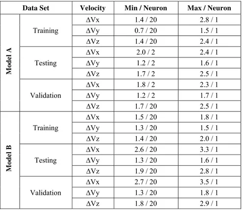
The significance of pruning away hidden neurons in BPANN architecture is investigated by RMSE values of the velocity residuals (∆VX,Y,Z) of the training, testing and validation points (Figure 3 in appendix). The minimum and maximum values of these RMSEs and the corresponding hidden neuron numbers are summarized in Table 1, in appendix.

The reference velocity fields (VX,Y,Z) of the study area that are generated from GPS observations and the velocity residual (∆VX,Y,Z) maps with regard to the smallest velocity differences of the testing and validation points (associated with 20 hidden neurons) computed by equation (4), are given in Figure 4, in appendix. The contour lines are drawn at 2-mm intervals on the velocity residual maps.

5. RESULTS AND CONCLUSIONS

The analysis of the RMSE values given in Appendix, Figure 3 reveals that the training data set, the testing data set and the validation data set are very similar. The differences between the RMSE values based on the training points, the testing points and the validation points are quite small. It can be considered that the training data set represents the possible variations in the study area well.

(10)

Yilmaz, M.

5 6 7 validation data sets are better in Model A. This suggests that the training data set of Model A was representative of the entire data source (testing and validation data sets) and Model A produced RMSE values that were consistent for training, testing and validation data sets.

The graphical presentations in Appendix, Figure 3 confirms that BPANN architectures provide the sufficient RMSE values of the point velocity residual that relates the sufficient positional accuracy for the source data (±3 cm for TNFGN points).

The objective of this study was to quantify the significance of removing away hidden neurons in BPANN architecture for estimating the densification point velocity. From the results of this study, the following remarks can be made:

(1) The employment of BPANN with 30 hidden neurons did not lead an overfitting of data nor poor generalization. 30 hidden neurons is an acceptable value for starting removal processes of hidden neurons.

(2) Hidden neurons between 30 and 20 did not have a marginal effect on the resulting performance of BPANN.

(3) In Model A and Model B, minimum RMSE values (Model A→ ±1.4, ±0.7, ±1.4 mm/year; Model B → ±1.5, ±1.3, ±1.4 mm/year, respectively) of the training point velocity residuals are obtained by BPANN with 20 hidden neurons such as submitted by Gullu et al. (2011a) and by Yilmaz (2012).

(4) In Model A, sufficient RMSE values (±2.3, ±1.3, ±1.7 mm/year for the testing points; ±2.0, ±1.2, ±1.7 mm/year for the validation points, respectively) are estimated when 20 hidden neurons are used for BPANN architecture, with respect to the training set results.

(5) In Model B, minimum RMSE values (±2.6, ±1.3, ±1.9 mm/year for the testing points; ±2.7, ±1.3, ±1.8 mm/year for the validation points, respectively) are obtained by BPANN with 20 hidden neurons.

(6) The velocity residual (∆VX,Y,Z) maps in Appendix, Figure 4 clarify that BPANN architecture with 20 hidden neurons is effective for geodetic velocity field determination with a satisfactory positional accuracy.

(7) In Model A, BPANN with 2 hidden neurons provided the smallest RMSE values (±2.0, ±1.2, ±1.7 mm/year for the testing points, respectively) of the velocity residuals (associated with ∆VX,Y,Z) and (±1.8, ±1.2 mm/year for the validation points, respectively) of the velocity residuals (associated with ∆VX,Y). For the training data set, RMSE values (±1.7, ±1.1, ±1.6 mm/year, respectively) are obtained by the same BPANN architecture.

(8) Maximum RMSE values of the velocity residuals for all three data sets are obtained by BPANN with 1 hidden neuron in Model A and Model B. These results show that BPANN could not learn the source data sufficiently and accurately when the number of hidden neurons is 1 (Nh<N).

(11)

5 6 8

used in velocity field determination. 20 hidden neurons can be accepted as a starting value in the pruning approach with a training set that distributes throughout the study are in all dimensions (representative of the testing and validation data sets). Furthermore, a rough guideline of appropriate number of hidden neurons can be introduced as Nh ≤T with respect to the accuracy of the result and the learning time for adaptation of BPANN for estimating the geodetic point velocities, determining velocity field in locations where future GPS stations could be deployed and interpolating the velocity field in areas that will not be instrumented.

ACKNOWLEDGEMENTS

The author thanks the two anonymous reviewers for their constructive comments to the paper.

REFERENCES

ALDRICH, C.; VAN DEVENTER, J.S.J.; REUTER, M.A. The application of neural nets in the metallurgical industry, Minerals Engineering, 7, 793-809, 1994.

BAILEY, D.L.; THOMPSON, D.M. Developing neural-network applications, AI Expert, 5 (9), 34-41, 1990.

BARRON, A.R. Approximation and estimation bounds for artificial neural networks, Machine Learning, 14 (1), 115-133, 1994.

BEALE, M.H.; HAGAN, M.T.; DEMUTH, H.B. Neural Network Toolbox 7 User’s Guide. The MathWorks Inc., Natick, MA, 951 pp., 2010.

BISHOP, C.M. Neural networks for pattern recognition, Oxford University Press, New York, NY, 482 pp., 1995.

CYBENKO, G. Approximations by superpositions of sigmoidal functions,

Mathematics of Control, Signals and Systems, 2 (4), 303-314, 1989.

D'ANASTASIO, E.; DE MARTINI, P.M.; SELVAGGI, G.; PANTOSTI, D.; MARCHIONI, A.; MASEROLI, R. Short-term vertical velocity field in the Apennines (Italy) revealed by geodetic levelling data, Tectonophysics, 418, 219-234, 2006.

FERLAND, R.; ALTAMIMI, Z.; BRUYNINX, C.; CRAYMER, M.; HABRICH, H.; KOUBA, J. Regional networks densification, IGS Workshop Towards Real-Time, Ottawa, Canada, pp. 123-132, 2002.

FUNAHASHI, K. On the approximate realization of continuous mappings by neural networks, Neural Networks, 2, 183-192, 1989.

GULLU, M.; YILMAZ, I.; YILMAZ, M.; TURGUT, B. An alternative method for estimating densification point velocity based on back propagation artificial neural networks, Studia Geophysica et Geodaetica, 55 (1), 73-86, 2011a. GULLU, M.; YILMAZ, M.; YILMAZ, I. Application of back propagation artificial

(12)

Yilmaz, M.

5 6 9 HAYKIN, S. Neural networks: A comprehensive foundation, Prentice Hall, Upper

Saddle River, NJ, 842 pp., 1999.

HEFTY, J. Densification of the central Europe velocity field using velocities from local and regional geokinematical projects, Geophysical Research Abstracts, 10 (EGU2008-A-01735), 2008.

HOLMSTROM, L.; KOISTINEN, P. Using additive noise in back-propagation training, IEEE Transactions on Neural Networks, 3 (1), 24-38, 1992.

HORNIK, K.; STINCHCOMBE, M.; WHITE, H. Multilayer feedforward networks are universal approximators, Neural Networks, 2, 359-366, 1989.

KAASTRA, I.; BOYD, M. Designing a neural network for forecasting financial and economic time series, Neurocomputing, 10, 215-236, 1996.

KANELLOPOULAS, I., WILKINSON, G.G. Strategies and best practice for neural network image classification, International Journal of Remote Sensing, 18 (4), 711-725, 1997.

KARIMI, S.; KISI, O.; SHIRI, J.; MAKARYNSKYY, O. Neuro-fuzzy and neural network techniques for forecasting sea level in Darwin Harbor, Australia,

Computers and Geosciences, 52, 50-59, 2013.

KATZ, J.O. Developing neural network forecasters for trading, Technical Analysis of Stocks and Commodities, 10 (4), 160-168, 1992.

LAAR, P.V.D.; HESKES, J. Pruning using parameter and neuronal metrics, Neural Computation, 11, 977-993, 1999.

LEANDRO, R.F.; SANTOS, M.C. A neural network approach for regional vertical total electron content modelling, Studia Geophysica et Geodaetica, 51 (2), 279-292, 2007.

LE CUN, Y.; DENKER, J.; SOLLA, S.; HOWARD, R.E.; JACKEL, L.D. Optimal brain damage, In: TOURETZKY, D.S. (Ed.), Advances in Neural Information Processing Systems II, Morgan Kauffman, San Francisco, CA, pp. 598-605, 1990.

LIANG, X. Removal of hidden neurons in multilayer perceptrons by orthogonal projection and weight crosswise propagation, Neural Computing and Applications, 16, 57-68, 2007.

LIU, Y.; STARZYK, J.A. Optimized approximation algorithm in neural networks without overfitting, IEEE Transactions on Neural Networks, 19 (6), 983-995, 2008.

MAHMOUDABADI, H.; IZADI, M.; MENHAJ, M.B. A hybrid method for grade estimation using genetic algorithm and neural networks, Computers and Geosciences, 13, 91-101, 2009.

MOGHTASED-AZAR, K.; ZALETNYIK, P. Crustal velocity field modelling with neural network and polynomials, In: SIDERIS, M.G. (Ed.), Observing our changing Earth, International Association of Geodesy Symposia, 133, pp. 809-816, 2009.

(13)

5 7 0

NOCQUET, J.M.; CALAIS, E. Crustal velocity field of western Europe from permanent GPS array solutions, 1996–2001, Geophysical Journal International, 154, 72-88, 2003.

NØRGAARD, M. Neural Network Based System Identification Toolbox, Technical

Report 97-E-851, Department of Automation Technical University of

Denmark, Copenhagen, Denmark, 31 pp., 1997.

PANCHAL, G.; GANATRA, A.; KOSTA, Y.P.; PANCHAL, D. Behaviour analysis of multilayer perceptrons with multiple hidden neurons and hidden layers,

International Journal of Computer Theory and Engineering, 3 (2), 332-337, 2011.

PANDYA, A.S.; MACY, R.B. Pattern recognition with neural networks in C++,

CRC Press, Boca Raton, Florida, 410 pp., 1995.

REED, R. Pruning algorithms - a survey, IEEE Transactions on Neural Networks, 4 (5), 740-747, 1993.

REZAEI, K.; GUEST, B.; FRIEDRICH, A.; FAYAZI, F.; NAKHAEI, M.; BEITOLLAHI, A.; FATEMI-AGHDA, S.M. Feed forward neural network and interpolation function models to predict the soil and subsurface sediments distribution in Bam, Iran, Acta Geophysica, 57 (2), 271-293, 2009.

SAVIO, A.; CHARPENTIER, J.; TERMENON, M.; SHINN, A.K.; GRANA, M. Neural classifiers for schizophrenia diagnostic support on diffusion imaging data, Neural Network World, 20 (7), 935-950, 2010.

SINGH, N.; SINGH, T.N.; AVYAKTANAND, T.; KRIPA, M.S. Textural identification of basaltic rock mass using image processing and neural network, Computers and Geosciences, 14, 301-310, 2010.

TEOH, E.J.; TAN, K.C.; XIANG, C. Estimating the number of hidden neurons in a feedforward network using the singular value decomposition, IEEE Transactions on Neural Networks, 17 (6), 1623-1629, 2006.

TURKISH CHAMBER OF SURVEY AND CADASTRE ENGINEERS. Large scale map and map information Production regulation [in Turkish], Iskur Press, Ankara, 260 pp., 2008.

WITTEN, I.H.; FRANK, E. Data mining: Practical machine learning tools and techniques, Morgan Kaufmann, San Francisco, CA, 560 pp., 2005

WRIGHT, T., WANG, H. Large-scale crustal velocity field of western Tibet from InSAR and GPS reveals internal deformation of the Tibetan plateau,

Geophysical Research Abstracts, 12 (EGU2010-7092), 2010.

YILMAZ, M. The Utility of Artificial Neural Networks in Geodetic Point Velocity Estimation [in Turkish], Ph.D. Dissertation, Afyon Kocatepe University, Afyonkarahisar, Turkey, 106 pp., 2012.

ZHANG, G.; PATUWO, B.E.; HU, M.Y. Forecasting with artificial neural networks: The state of the art, International Journal of Forecasting, 14, 35-62, 1998.

(14)

Y Yilmaz, M.

Figure

Bol. Ci 3 - RMSE val

iênc. Geod., sec. APP

lues of the trai

Artigos, Curitiba PENDIX

ining, testing

a, v. 19, no_{4, p.55}

and validation

58-573, out-dez, 2 5

n data sets.

(15)

5 7 2

Table 1 - The minimum and maximum values of RMSEs (in mm/year).

Data Set Velocity Min / Neuron Max / Neuron

Mo

del A

Training

∆Vx 1.4 / 20 2.8 / 1

∆Vy 0.7 / 20 1.5 / 1

∆Vz 1.4 / 20 2.4 / 1

Testing

∆Vx 2.0 / 2 2.4 / 1

∆Vy 1.2 / 2 1.6 / 1

∆Vz 1.7 / 2 2.5 / 1

Validation

∆Vx 1.8 / 2 2.3 / 1

∆Vy 1.2 / 2 1.7 / 1

∆Vz 1.7 / 20 2.5 / 1

Mo

del B

Training

∆Vx 1.5 / 20 1.8 / 1

∆Vy 1.3 / 20 1.5 / 1

∆Vz 1.4 / 20 2.0 / 1

Testing

∆Vx 2.6 / 20 3.3 / 1

∆Vy 1.3 / 20 1.6 / 1

∆Vz 1.9 / 20 2.8 / 1

Validation

∆Vx 2.7 / 20 3.5 / 1

∆Vy 1.3 / 20 1.8 / 1

(16)

Yilmaz, M.