WEEKLY TRACKING OF STABILITY OF THE
FLOW OF CONVERSATIONS INTO THE
SUBPROCESSES OF LAST PLANNER SYSTEM
Omar Zegarra1, Luis Fernando Alarcón2, Pedro Pereira3 and Nuno Cachadinha4
ABSTRACT
The reliability of a Production Control System impacts productivity; research suggests that Last Planner System - reliability could be improved with a variability analysis and control of its subprocesses. The variability ratio of those subprocesses, known as the Bullwhip Effect of Conversations, helps to quantify the conversation flow between the Last Planner System subprocesses. We assessed if the first stages of the Bullwhip Effect of Conversations evaluation methodology could be used as a weekly tool, to measure the proper application of Production Control System - subprocesses. This paper reports the analysis of conversations trends, statistical controls and the impact of the Production Control System subprocesses using two case studies: one carried out in South America which used the Last Planner System, and one in Europe which used the Traditional Production Control System. We found production control subprocesses which were under statistical control, and that impact one another as well as the PPC. With this methodology, it is possible to evaluate the stability of the coordination flows into each Production Control System - subprocesses. Both cases were stable, predictable and free of external causes of variation. We consider that this method could be valuable for tracking and tuning the application of Last Planner System subprocesses.
KEYWORDS
Last Planner, Production Planning, Control, Variability, Language Action Perspective.
INTRODUCTION
A Production Control System (PCS) is used to set conditions to manage project operations. From the point of view of Lean Construction, the application of a PCS while using traditional management methods could result in inadequate control given that a Traditional Production Control (TPC) System is based on a project control model (Koskela and Ballard 2006). The Last Planner System (LPS) was introduced to address this situation (Ballard et al 1998). According to the literature, its use
1
PhD Candidate and Graduate Researcher at Centro de Excelencia en Gestión de Producción (GEPUC) at Pontificia Universidad Católica de Chile. E-mail:[email protected], (56 2) 354-4244
2
PhD, Head Professor, Dep. of Construction Management Pontificia Universidad Católica de Chile, E-mail: [email protected], (56 2) 354-4201, (56 2) 354 4244.
3
Graduate Researcher, Dep. de Eng. Civil, Dept of Science and Technology, Universidade Nova de Lisboa, 351 212 948 557 E-mail: [email protected]
4
positively affects the safety, productivity and cost of construction operations (Alarcón & Leal 2010).
A PCS involves the use of a sequence of management processes prior to the successful execution of physical operations, both for LPS and TPC. In the LPS, the successful completion of these sub processes is evaluated by the Percent Plan Complete (PPC) index, but so far, it has not been reported a method to evaluate ,strategically, the proper functioning of each of the PCS elements. Unstable PCS subprocesses could propagate variability along PCS process and to the physical operations.
To address the previous issue, the Bullwhip of Conversations (BWE) concept (Alarcón and Zegarra, 2012) was developed. It seeks to quantify the behavior of the variability along the PCS subprocesses. To use this concept, a key first step is the evaluation of the stability of the PCS subprocesses, i.e. if the mean and dispersion change abruptly due to special causes of variation (which must be detected and eliminated).
In this paper we have evaluated the feasibility of using the first stages of the BWE evaluation methodology as a tool for weekly tracking of the proper use of PCS subprocesses. This means to identify if we can use them, and how they should be used on a regular basis to approach the control of stability of PCS subprocesses. To do so, we have studied the stability of PCS subprocesses of two construction projects: one carried out in South America and one in Europe. One of them uses the LPS and the other a TPC (the latter has been expressed in LPS terms in order to make the comparison).
LITERATURE REVIEW
BACKGROUND
Conversations & Language Action Perspective (LAP) (Flores & Ludlow 1982). - The LAP theory describes a process of interaction between people based on the use of language and actions to perform some activity, i.e. acts of speech. Some key ideas within it are: (1) Conversation (a sequence of acts of speech and milestones), (2) Requirements and Promises (they are types of acts of speech), and (3) Articulation of Conversations (a management process, based on the generation and articulation of commitments). The literature also suggests that LAP allows effective, articulate conversion, which results in positive LPS results (Macomber and Howell 2005).
Bullwhip Effect (Forrester 1961, Lee 1997). - The Bullwhip Effect has been defined as the propagation of variability of information flows and physical stocks along a supply chain. This phenomenon deteriorates the performance of a system. This is inevitable because it arises from the structure of the system itself. The differences between this concept and the BWE are based on the use of the concept of conversations and pull PCS (Zegarra & Alarcon 2013).
Bullwhip of Conversations (BWE) (Alarcón & Zegarra 2012). - Its features are:
Existence and Impact: The research cited documents this concept existence in real cases and its effect on reliability. The study checked for BWE indexes that: (1) During the LPS process there are values > 1 (i.e. they exists) and (2) they affect PPC.
Evaluation Process: It considers three stages (each one is an input to the next): (1) Measurement of conversations, (2a) Qualitative analysis and (2b) Quantitative analysis. Each stage´s targets are: (1)To count the weekly conversations within each LPS variable, (2a) to evaluate the conversations variability within each LPS variable and (2b)to assess the variability propagation by calculating BWE indexes between LPS variables.
Figure 1. Mechanism that produces the BWE of Conversations (Alarcón & Zegarra, 2012)
Notes: Stock of conversations within LPS variables
Flow of conversations between LPS variables LPS subprocesses: M, LA, C, W and RNC
STAGE 1&2A: MEASUREMENT AND QUALITATIVE ANALYSIS OF CONVERSATIONS
(ALARCON &ZEGARRA 2012)(ZEGARRA 2012)
These stages follow the logic of a time series modelling, with a statistical process control of the residuals. (Brockwell and Davis 2002; Cachon et al 1997; NIST / SEMATECH 2012) Their goals include: (1) to assess trends and stationarity of data for each LPS variable, (2) to remove trends to get stationary residuals (i.e. to find outliers), (3) to evaluate the existence of special causes of variation. In practical terms, these stages count the weekly conversations into each LPS variable, transform them to data series of rates of change (%) and evaluate its variability. The process has the following steps:
(1) Identification of trends. - Detects the existence of trend changes and scale variation in the data series (i.e. find if are stationary). The trend is calculated using a moving average. The lack of stationarity constraints the direct assessment of relationships between data sets, because it can generate spurious relationships.
(2) Elimination of Trend. - In order to use a conversations data series that presents non- stationary behavior and heteroscedasticity (changing variability over time),it is necessary to use a mathematical transformation process based on (a) logarithms use and (b) successive differentiation of quantities.
(3) Identification of Residuals or Change (%). - The transformation output is a data series of statistic residuals. They are characterized by being linear, with regular variability, useful to discover trends and outliers; because of the two transformation techniques used, this value also represents a relative change between two successive readings. The relationships identified between two change (%) series also describe the relationship between the original series (Nau 2005).
existence: (1) Shewhard (i.e. points outside a 3 sigma limit) and (2) Western Electric Company-WECO tests (NIST/SEMATECH 2012) (see Appendix).
(5) Definitions (Zegarra & Alarcon 2013). - The measurements considered are: (1) Residual = Change (%) (Nau 2005); (2) Change (%) = weekly flow rate of conversations within each LPS variable (this is different to flow rate of conversations between LPS variables, e.g. the flow of Master (M) to Look Ahead (LA),i.e. the transformation of M into LA) ; (3) Conversations Flow Rate within each LPS variable = Coordination flow rate (it has been suggested that the conversations flow describes the coordination process (Zegarra & Alarcon 2013), i.e. management of dependencies between elements; e.g. Within the LA variable, the conversations flow describes the coordination at the LA planning level to change the LA stock); and (4)Stability of Coordination = Regular Adaptation (i.e. if stability is observed, it suggests the existence of capability to keep on a regular adaptation to new conditions imposed by the project´s changing conditions).
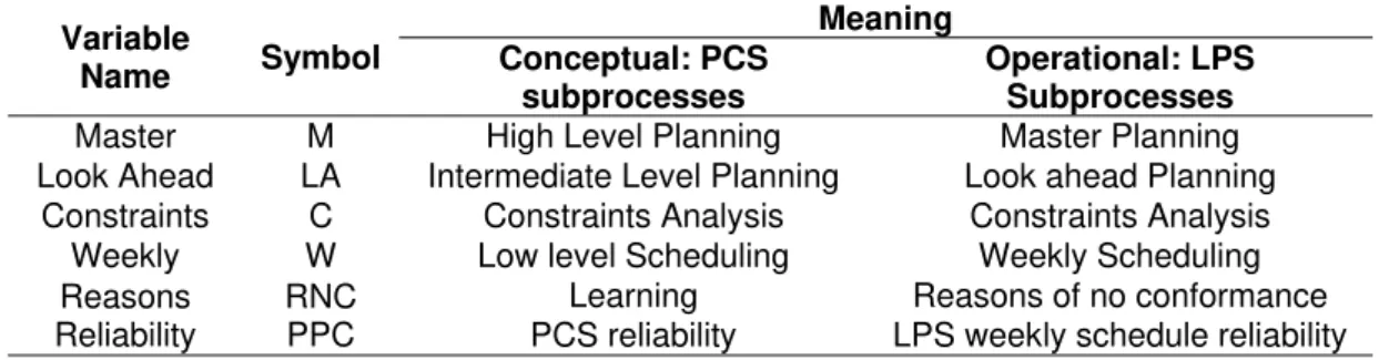
Table 1 Hypothesis Variables Dictionary
Variable
Name Symbol
Meaning Conceptual: PCS
subprocesses
Operational: LPS Subprocesses
Master M High Level Planning Master Planning
Look Ahead LA Intermediate Level Planning Look ahead Planning
Constraints C Constraints Analysis Constraints Analysis
Weekly W Low level Scheduling Weekly Scheduling
Reasons Reliability
RNC PPC
Learning Reasons of no conformance
PCS reliability LPS weekly schedule reliability
HYPOTHESES
To carry out this research, we considered the following hypotheses and variables (Table 1): (H1) PCS subprocesses are stable in the LPS; (H2) PCS subprocesses are not stable in the TPC and (H3) PCS subprocesses stability impacts PPC stability
METHODOLOGY
To evaluate the hypothesis of this study, we used a case study strategy. It included the use of information from two projects: one conducted in South America (Alarcón and Zegarra, 2012) and the other one in Europe (Pereira et al, 2013). The method used to calculate the stability of the PCS subprocesses corresponds to steps 1 and 2a of the BWE/LPS measurement method. Finally, the output of the stages was assessed, and it included the impact of PCS variables variability on each other and on the PPC variability.
Table 2 Case Characteristics & Baseline Information
CASE 1: 100 KM Road
Maintenance: Quarry Works, Aggregate Processing, Surface Treatments (fog Seal, Chip Seal), Signalization.
CASE 2: Modernization and rehabilitation of a naval
shipyard: Repair of concrete floor slabs, panels and top wall beam of slurry walls, joint sealing and finishing, earth works, installation of electrical
distribution chambers and electrodes, rehabilitation of draining pits and galleries and sewage works.
Cases - this paper used two case studies (Table 2). Case A was conducted in Peru and the project used LPS; case B was carried out in Portugal and used a TPC; in order to make a comparison, case B was expressed in terms of LPS. The feasibility of this consideration was reviewed in Pereira et al 2013.
Process - the analysis considered the following steps (Alarcon & Zegarra, 2012): Stage 1 Collection and Quantification: (1) Weekly data organization; (2) Quantification of weekly conversations within each LPS variable; (3) Construction of original time series -for each LPS variable-.
Stage 2a Qualitative Analysis: (1) Variability Filtering (calculating moving averages for three consecutive values). (2) Residuals Identification (logarithmic transformation and differentiation –i.e. homogenization of variability, trend removal, and calculating the relative exchange rate-) (3) Stability Evaluation (assessment of dynamic behaviour and statistical control of residuals).
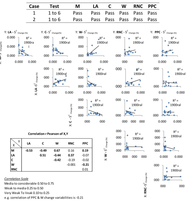
Stage 3 Relationship of Qualitative Analysis Output and Reliability: (1) the variance of change for three consecutive weeks (starting week 3) were used to relate PCS sub process with each other and with PPC. To do this, scatter plots and the r Person coefficient between variances of LPS variables were used.
RESULTS
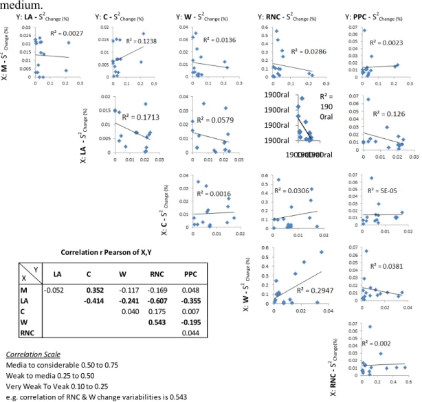
The results of this analysis for hypotheses H1 and H2 can be seen in Figure 2 (Time Series and Trend), Figure 3 (Weekly rate of change (%)) and Table 3 (Evaluation of Stability). For the hypothesis H3, the results are exhibited in the Figure 4 (Case 1), and Figure 5 (Case 2); these figures present the comparison of variances (of weekly % change) of the PCS subprocesses and the PPC.
Figure 2: In cases A and B, all variables present location and scale change. In both cases, the PPCs exhibit an upward trend. In general, the PCS subprocesses (expressed in terms of LPS variables) present decreasing trends.
Table 3 (It evaluates Figure 3): Cases A and B have, in general, all the LPS variables under statistical control. Each variable passed the Shewhard and WECO tests.We observed only two points out of control, one in the Weekly Schedule (W) (i.e. it failed test 3 of WECO for weeks 11 to 13 ) and one in Reasons of no conformance
(RNC) in Case 2.
Figure 4: The Pearson coefficient between change variances, suggests a considerable impact of Master (M) on Look Ahead (LA), Constraints(C), and W, LA on C and W, and C on W. The effect on PPC is weak; M & W affect PPC the most.
Figure 5: The Pearson coefficient between change variances suggests, that there is a considerable impact of LA and Won RNC; and a weak- to- medium impact of M on C, of LA on C & PPC; LA & W affect PPC the most.
ANALYSIS
criteria; both cases suggest isolated incidents and temporary out-of-control situations that were corrected.
CASE 1 CASE 2
M LA M LA
Conversations
C W C W
Conversations
RNC PPC RNC PPC
Conversations
Weeks Weeks Weeks Weeks
Figure 2. Run Charts (-) and Trends () of LPS Conversations and LPS Reliability (PPC)
CASE 1: Statistical Control** CASE 2: Statistical Control**
Conv. Chan ge (%)
M LA M LA
Conv. Chan ge (%)
C W C W
Conv. Chan ge (%)
RNC PPC RNC PPC
Weeks Weeks Weeks Weeks
Figure 3. Change (%) of Conversations & PPC ** limits: 1 [ __ ], 2[---] & 3 [- ] Standard Dev. 1900ral
1900ral 1900ral
1 6 11 16
1900ral 1900ral 1900ral
1 6 11 16
1900ral 1900ral
1900ral 1900ral
1 6 11 16
1900ral 1900ral 1900ral 1900ral
1 6 11 16
1900ral 1900ral
1 6 11 16
1900ral 1900ral
1 6 11 16
1900ral 1900ral
1 6 11 16
1900ral 1900ral
1 6 11 16
0% 100%
1 6 11 16
1900ral 1900ral
1 6 11 16
0% 100%
1 6 11 16
000 000 000
1 6 11 16
000 000 000
1 6 11 16
‐,700
‐,350
,000 ,350 ,700
1 6 11 16
‐,400
‐,200
,000 ,200 ,400
1 6 11 16
‐001
000 001
1 6 11 16
000 000 000 000 000
1 6 11 16
‐,400
‐,200
,000 ,200 ,400
1 6 11 16
‐,300
‐,150
,000 ,150 ,300
1 6 11 16
000 000 000 000 000
1 6 11 16
000 000 000 000 000
1 6 11 16
‐1,200
‐,600
,000 ,600 1,200
1 6 11 16
‐,500
‐,250
,000 ,250 ,500
Table 3. Evaluation of Statistical Tests of Shewhard &WECO
Case Test M LA C W RNC PPC
1 1 to 6 Pass Pass Pass Pass Pass Pass
2 1 to 6 Pass Pass Pass Pass Pass Pass
X: M ‐ S 2 Ch a n ge( % )
Y: LA ‐ S2 Change (%) Y: C‐ S2 Change(%) Y: W‐ S2 Change (%) Y: RNC ‐ S2 Change (%) Y: PPC ‐ S2 Change (%)
X: LA ‐ S
2 Ch
a n ge (% ) X: C ‐ S
2 Ch
a n ge (% ) X: W ‐ S
2 Ch
a n ge (% ) X: RNC ‐ S 2 Ch a n g e (%)
Figure 4. Case 1: Impact of PCS variables into each other and into PPC - relationship of variances of change (%) -
Hypothesis H3.- In Case 1, with higher PPC index, a strong relationship was found within the first group of LPS variables (between its variances of change); it seems that the LPS subprocesses put emphasis on the proactive action rather than on problem solutions . What was not expected is the low relationship with the PPC change variances. In Case 2, with comparative lower PPC index, stronger relationships were observed in the relationship of LA and W with RNC (between its variances of change); maybe it suggests that this second case had to struggle more with unexpected problems. Also the impact of LA along all the process is remarkable.
R² = 1900ra l 0.000 0.000 0.000 0.000 0.000
R² = 1900ral
000 000 000
0.000 0.000
R² = 1900ral
000 000 000
0.000 0.000
R² = 1900ral
000 000
000 000
R² = 1900ral
000 000
0.000 0.000
R² = 1900ral
000 000 000
0.000 0.000
R² = 1900ral
000 000 000
0.000 0.000
R² = 1900ral
000 000
0.000 0.000
R² = 1900ral
000 000
0.000 0.000
R² = 1900ral
000 000 000
000 000
R² = 1900ral
000 000
000 000 000
R² = 1900ral
000 000
0.000 0.000
LA C W RNC PPC
M ‐0.53 ‐0.49 0.67 0.16 0.19
LA 0.51 ‐0.44 0.37 ‐0.07
C ‐0.42 ‐0.19 ‐0.02
W ‐0.001 ‐0.21
RNC 0.01
Correlation Scale
Media to considerable 0.50 to 0.75
Weak to media 0.25 to 0.50
Very Weak To Veak 0.10 to 0.25
e.g. correlation of PPC & W change variabilities is ‐0.21
Correlation r Pearson of X,Y
X Y
R² = 1900ral
000 000 000 000
000 000 000
R² = 1900ral 000 000 000 000 0.000 0.000
R² = 1900ral
000 000
Again in this case the relationship with PPC change variances was at most weak- to- medium.
X:
M
‐
S
2 Ch
a
n
ge
(%
)
Y: LA ‐ S2Change (%) Y: C ‐ S2Change (%) Y: W‐S2Change (%) Y: RNC‐S 2
Change (%) Y: PPC ‐ S 2
Change (%)
X:
LA
‐
S
2 Ch
a
n
g
e
(%)
X:
C
‐
S
2 Ch
a
n
ge
(%
)
X:
W
‐
S
2
Ch
a
n
ge
(%
)
X:
RNC
‐
S
2 Ch
a
n
ge(
%
)
Figure 5. Case 2: Impact of PCS variables into each other and into PPC - relationship of variances of change (%) -
Also in both cases, despite the different PCS use, the tendencies presented similar behaviors, which in general is downward. The differences in the trends of M describe how the project has been managed; In the case 2, the scope presented several updates The case of LA shows a slightly decreasing trend; the case of C observed a downward trend (although case 1 has a significant swing in the middle); In the case of W and RNC, the trend is a very clear downward one; The PPC trends suggest an upward behavior. Although, the trends may suggest that, as the quantity of conversations required for the project is reduced, the reliability is increased, this condition is not observed in the correlation analysis of variances of change, i.e. some variables increase it and others reduce it.
DISCUSSION
This analysis evaluates the use of one part of a methodology of variability analysis as a weekly tool, and its effect on planning reliability, based on the analysis of two PCS systems. The analysis suggests that Hypothesis H1 would be true, while H2 and H3
R² = 190 0ral
1900ral 1900ral 1900ral 1900ral
1900ral1900ral1900ral
LA C W RNC PPC
M ‐0.052 0.352 ‐0.117 ‐0.169 0.048 LA ‐0.414 ‐0.241 ‐0.607 ‐0.355
C 0.040 0.175 0.007
W 0.543 ‐0.195
RNC 0.044
Correlation Scale
Media to considerable 0.50 to 0.75 Weak to media 0.25 to 0.50 Very Weak To Veak 0.10 to 0.25
e.g. correlation of RNC & W change variabilities is 0.543 Correlation r Pearson of X,Y
are false. That is, the LPS and TPS sub processes are under statistical control, since both do not exhibit special causes of variation. In the case of H3, although a certain level of relationship exists with the PPC change variance, it is not strong. The implications are discussed below.
Project Assessment: It is plausible to suggest, based on the statistical control observed, that both PCS were carried out acceptably. In the case of LPS, this can be attributed to the systematic use of the method. In the case of TPC, this could be attributed to the use of adequate elements of control; although different from LPS, they have produced adequate results. This control level seems to explain the conversations´ downward trend, especially in LA, C, W and RNC and also it would be consistent with the increasing trend in the PPC.
Meaning: These assessments may describe the coordination within each PCS subprocess. The declining trends, especially, in W, C and RNC, in both projects, seem to suggest the development of a learning curve, which could be consistent with the existence of stable project coordination; i.e. the results delivered by the stability analysis, which suggests that the change (%) in all variables in both cases is regular; that is, there is no problem in adaptation to new circumstances originated in requirements set by the Master Plans.
Practical Use: It suggests that these measurements could be used in a practical way to determine whether the coordination is adapting to the changing conditions at an appropriate rate during the project, i.e. if management efforts are increasing in the right proportion to face an increasing number of activities during the project. In practical terms, this means trying to keep the rate of change (%) stable (or within statistic limits of control) while reducing -because of learning- the amount of conversations or while increasing the PPC
At the Project level, these kinds of measures could be useful for project control of production management processes. The use of (1) run charts & trends of conversations and (2) control charts of change (%) rates resemble the variation monitoring of an amount of money and its interest rate along a timeframe, where the money are the conversations and the interest is the rate of change (%) (i.e. the coordination effort). At the Company level, this measure seems appropriate for learning about the PCS used by the firm for projects.
Disadvantage: The limited relationship observed with PPC change variability raises questions about the utility of the stability analysis as a predictor of the PPC index; more research about it is required.
CONCLUSIONS AND RECOMENDATIONS
We consider that the use of these elements of the BWE/LPS methodology could be useful to track the stability of PCS subprocess changes (%) throughout the project. They could be used as a predictor of the behavior of other PCS subprocess, although it seems that they do not relate strongly with PPC change variability behavior.
Regarding the stability analysis, for both cases, all PCS subprocesses and PPC have been identified as stable and under statistical control. This means that the conversations behaviour do not have special causes of variation, that drives them beyond the natural limits of the PCS process.
plausible to say that team´s coordination is able to adapt at an appropriate rate to the changing conditions of the master schedule.
APPENDIX
Western Electric Company Rules (WECO)(NIST/SEMATECH 2012).- This stability criteria considers a process is unstable if any of the following six situations is present: (1) 8 consecutive points between center & +/-1 sigma;, (2) 4 out of last 5 points between +/-1 & +/-2 sigma; (3) 2 out of last 3 between +/-2sigma & +/-3 sigma; (4) any Point above +/-3 sigma; (5) trends of a 6 in a row going up or going down, (6) trends of 14 point in a row going up and down.
REFERENCES
Alarcon L.F. and Zegarra O. (2012), “Identifying the Bullwhip Effect of Last Planner Conversations during the Construction Stage”, IGLC-20, Berkeley,California. Ballard G . and Howell G. (1998) “ Shielding Production: Essential Step in
Production Control”, Journal of Construction Engineering and Management, Vol 124 Nro 1, 1998.
Brockwell P. and Davis R. (2004), Intro. to Time Series Forecasting, 2th Ed., Springer, U.S.
Cachon G.P., Randall T. and Schmidt G.M. (2007). “In Search of the Bullwhip Effect”, Manufacturing & Service Operations Management, 9(4), Fall, 457-479. Flores, F., J.J. Ludlow (1980), Doing and Speaking in the Office, In: G. Fick, H.
Spraque Jr. Eds., Decision Support Systems: Issues and Challenges, Pergamon Press, NY, pp95-118.
Forrester J. (1961), Industrial Dynamics, The MIT press, MIT, Cambridge, Massachusetts.
Koskela L. & Ballard G. (2006)”Should Project Management be based on theories of economics or production?.” Building and Research & Information 34(2), 154-163. Leal M. and Alarcon L.F. (2010). “Quantifying Impacts of Last Planner
Implementation in Mining Projects.”, IGLC-18, July 2010, Haifa, Israel.
Lee H.L., Padmanabhan V. And Whang Seungjin (1997)” The Bullwhip Effect in Supply Chains” Sloan Management Review, Spring1997, 93 – 102.
Macomber H. and Howell G. (2005). “ Linguistic Action: Constribution to the Theory of Lean Construction”. Proceedings IGLC – XX,
NIST/SEMATECH e-Handbook of Statistical Methods, http://www.itl.nist.gov/div898/handbook/ March 2013. Nau R (2005), Forecasting Course, Duke University,
http://people.duke.edu/~rnau/Decision411CoursePage.htm/March 2013
Pereira P., Cachandinha, N. Zegarra O. & Alarcón L.F. (2013), “Bullwhip in Production Control: A Comparison Between Traditional Methods and LPS” Submitted to IGLC 21, Fortaleza, Brazil.
Zegarra and Alarcon (2013), “Propagation and Distortion of Variability into the Production Control System: Bullwhip of Conversations in the Last Planner”, Submitted to IGLC 21, Fortaleza Brazil