ISSN 0104-6632 Printed in Brazil
www.abeq.org.br/bjche
Vol. 33, No. 01, pp. 155 - 168, January - March, 2016 dx.doi.org/10.1590/0104-6632.20160331s00001267
Brazilian Journal
of Chemical
Engineering
ADVANCED CONTROL OF A COMPLEX
CHEMICAL PROCESS
Roxana Both
1, Eva-Henrietta Dulf
1*and Ana-Maria Cormos
21Technical University of Cluj Napoca, Memorandumului St., No. 28, RO - 400014, Cluj-Napoca, Romania. 2
Babes-Bolyai University, Faculty of Chemistry and Chemical Engineering, Arany Janos St., No. 11, RO-400028, Cluj-Napoca, Romania.
Phone: + 40-264-401821; Fax: + 40-0264-401220 E-mail: [email protected]; http://aut.utcluj.ro
(Submitted: July 25, 2011 ; Revised: February 12, 2015 ; Accepted: February 21, 2015)
Abstract - Three phase catalytic hydrogenation reactors are important reactors with complex behavior due to the
interaction among gas, solid and liquid phases with the kinetic, mass and heat transfer mechanisms. A nonlinear distributed parameter model was developed based on mass and energy conservation principles. It consists of balance equations for the gas and liquid phases, so that a system of partial differential equations is generated. Because detailed nonlinear mathematical models are not suitable for use in controller design, a simple linear mathematical model of the process, which describes its most important properties, was determined. Both developed mathematical models were validated using plant data. The control strategies proposed in this paper are a multivariable Smith Predictor PID controller and multivariable Smith Predictor structure in which the primary controllers are derived based on Internal Model Control. Set-point tracking and disturbance rejection tests are presented for both methods based on scenarios implemented in Matlab/SIMULINK.
Keywords: Multivariable Smith Predictor; Internal Model Control; Hydrogenation process; Dynamic mathematical model.
INTRODUCTION
The industrial scale 2-ethyl-hexenal hydrogenation process produces 2-ethyl-hexanol oxo-alcohol, used as raw material for dioctyl-phthalate (DOP) or 2-ethylhexyl-phthalate (DEHP) production. DOP and DEHP represent around 50% of the global consump-tion in the producconsump-tion of poly(vinyl chloride) (PVC) (ICIS,2011;WRI,2009;SRI,2011).
Because the hydrogenation reaction is highly exo-thermic, the reactor output temperature is of great importance. Like most of chemical and petro-chemi-cal plants, the 2-ethyl-hexenal hydrogenation process presents large time delays and is multivariable by nature. For multivariable time delay processes, the control solution will revolve around a multivariable Smith Predictor. A very important step for the
multi-variable Smith Predictors is the decoupling of the process.
15 fi d se tw re p p m si se p p ch d v co th re su v th sc ch th p n se fo re (2 n p 2 to fr tr fr re th m o ly is R 56
ive and six esign, respe even the com wo control st epresent the
P
The 2-ethy lex, which ca hase in the main product ide-products econdary si resent both hase 2-ethy haracterized imensions o antage: the p omparison to he advantag eaction of 2 umption, sm
olumes of ca he impossibi
cale liquid p hemical indu he present wo An import layed by the ickel catalys en based on or the 2-ethy ecommended
Several res 2011) studie
ism. Hence, resent case 011): the tra o the gas-liqu rom the gas-ransport of r rom the liqu eactant adsor he chemical molecules; pr f the catalys yst surface to s expressed a
C H C
R
C O
H
A
present a m ctively IMC mparative sim
trategies are last part of th
ROCESS D
yl-hexenal hy an take place presence of t (2 ethyl-hex
like: n-but ide-reactions
advantages a yl-hexenal h by high ene of equipment possibility to o the gas pha es of the li 2-ethyl-hexe mall dimensio
atalyst. How ility of catal phase hydrog ustries and re
ork.
tant role in th e catalyst. Fo st deposited
the BASF li yl-hexenal hy d in specific searchers lik ed the hydro
the reaction study are (B ansport of hy uid interface -liquid interf reactants 2-e uid phase to rption to the l reaction b roduct desor st; the produ o the liquid p as follows (C
+ H2
R C H2 C H
R
B
Ro
multivariable C control des
mulation resu presented. T he paper.
DESCRIPTIO
ydrogenation e both in liqu
a catalyst a xanol), can a tanol or iso s. Technolog and disadvan hydrogenatio ergy consum t, but has an o regenerate ase hydrogen iquid phase nal are: low on of equipm wever, the ma
lyst regenera genation is p epresents the
he hydrogena or the presen on silica su icense. This ydrogenation literature (Sm ke Bozga (20
ogenation re n mechanism Bozga et al., ydrogen from e; the transpo face to the li ethyl-hexenal o the active sites between ads rption from uct transport phase. The re Collins et al.,
H 2 + H C O
H R
oxana Both,
Eva-PID contro sign. In sect ults between The conclusio
ON
process is co uid phase or and, besides also form ot o-butanol fr gical solutio ntages. The on reaction mption and gr
n important the catalyst. nation reacti hydrogenat w energy c ment, and sm
ain drawback ation. Indust
predominant e main focus
ation reaction nt case study upport was c
type of catal reaction is a melder, 1989 001) and Coc
eaction mec m stages for , 2001; Cock m the gas ph
ort of hydrog quid phase; l and hydrog
solid interfa of the cataly sorbed react
the active si from the ca eaction pathw
2009):
R C H2 C H
R
C H2
C
-Henrietta Dulf an
ller tion the ons om-gas the ther rom ons gas is reat ad-. In ion, tion on-mall k is rial t in s of n is y, a ho-lyst also 9). cker cha-the ker, hase gen the gen ace; yst; tant ites ata-way wh hex hex sec pro tem rat hex to exo kca sid rea ord cal the lys tai dil its flo pro Fig hex pla po hy tur flo rec tai and me a d rea pro of O H
nd Ana-Maria Co
here: A is 2-xanal (inter xanol (final p
The main p cutive hydro oduct being mperature (i te and purity xenal). The t
the fact that othermic wi al/kmol (Sm de-reactions,
actants betw der to start th l recommend e range of 16 st degree of n the tempe lution of the elf (the refl ow diagram ocess is pres
gure 1: Proc xenal hydro ants.
As presente rtance is the ydrogenation re. It was det ow ratio betw
circulated 2 ned to carry d also to ma ended range. disturbance b action and im oduct. The n
a decrease ormos -ethyl-hexena rmediate pro product). parameters th ogenation re g 2-ethyl-hex input/output) y of input rea temperature t the hydrog ith a reacti melder,1989). but also an ween 90°C an
he reaction. T ded temperat 60 °C – 180 °
activity. The erature below
2-ethyl-hexa ux rate). A of the 2-eth ented in Figu
cess flow dia ogenation pr
ed before, a e reactor loa reaction its termined exp ween the 2-e -ethyl-hexan out the reac aintain the t The catalys because it inf mplicitly the necessary ste
in the cataly
al (reactant), oduct) and
hat influence eactions (the xanal) are: ), reactor lo actants (hydr
is a critical genation reac
on heat of . High temp n input temp nd 110°C is The maximu ture inside th °C, dependin e solution ch w the critica anal flow wi typical indu hyl-hexenal h
ure 1.
agram of a ty rocess used
a parameter ading. This self and also perimentally ethyl-hexenal nol flow mu ction with go
temperature st degree of a
fluences the h output temp eps to counte
yst activity a
, B is 2-ethy C is 2-ethy
e the two co e intermedia the pressur oading, reflu rogen, 2-ethy parameter du ction is high
25.27 x 1 peratures fav perature of th
s necessary um technolog he reactor is ng on the cat hosen to mai al value is th
ith the produ ustrial proce hydrogenatio
ypical 2-ethy in industri
of great im influences th o the temper
that a specif l flow and th ust be mai ood paramete in the recom activity acts
hydrogenatio perature of th eract the effe
the flow ratio (the recirculated 2-ethyl-hexanol flow must be decreased) and also to increase the input temperature of the reactants to start the hydrogena-tion reachydrogena-tion.
At the present time, the hydrogenation reactor is operated using an open loop control system, so the main parameters like 2-ethyl-hexenal input flow rate, recirculated 2-ethyl-hexanol flow and input tem-perature of the reactants are maintained at the im-posed values, without feedback control of output temperature or 2-ethyl-hexanol output concentra-tion. This control solution is characterized by a main disadvantage: it is not fault-tolerant, being difficult to apply correction methods if one control loop fails. However, the hydrogenation reactor will operate in a satisfactory manner if the auxiliary control loops for flow control of the reactants and input temperature control of the reactants are work-ing in good parameters.
At present an operator sets manually the reference values for the 2-ethyl-hexenal input flow rate, recir-culated 2-ethyl-hexanol flow and input temperature of the reactants. The 2-ethyl-hexanol output concen-tration is measured periodically and, if it is not satis-factory, the reference values for the main input varia-bles are adjusted by the accumulated expertise of the operator. In order to optimize the production, the authors propose a feedback control system using the existing infrastructure. The implementation costs are reduced to the costs of a temperature transducer used to measure the output temperature of the product.
In order to ensure safe and normal conditions of operation for the hydrogenation process there are two main goals of the control strategy. The first goal is to maintain the temperature at an acceptable value. This goal can be achieved by assuring a specific volumetric flow ratio between the 2-ethyl-hexenal and 2-ethyl-hexanol flow rates. The recirculated 2-ethyl-hexanol flow rate is considered to be the ma-nipulated variable. The second goal is to ensure a high conversion of 2-ethyl-hexenal to 2-ethyl-hexa-nol. This goal can be reached by assuring the neces-sary input temperature of the reactants to start the reaction. The input temperature of the reactants must be increased as the catalyst degree of activity decreases in time. The input temperature of the reactants also has an important influence on the output temperature. Overall, the two considered control inputs are the 2 ethyl-hexanol flow rate and the input temperature of the reactants. The output temperature and product concentration are consid-ered to be the measured outputs and the input hy-drogen pressure (P), and 2-ethyl-hexenal flow (Qenal) act as disturbances.
MATHEMATICAL MODELS
Distributed Parameter Nonlinear Mathematical Model
An accurate mathematical model is needed to evaluate the operational challenges and to understand the processes that occur inside the reactor and also to develop a more efficient control strategy. In the spe-cific literature, a number of kinetic studies of the hydrogenation reaction are reported (Smelder, 1989; Niklasson, 1987, 1988). However, no mathematical model of the process is given.
Motivated by these reasons, in previous works (Both, 2013), a first principle based mathematical model was developed starting only from some equa-tions describing the hydrogenation reaction kinetics. The developed model (Both, 2013), consisting of numerous partial differential equations and several algebraic ones, was implemented and validated using plant data acquired courtesy of S.C. Oltchim S.A. This model is useful in the design, optimization and operation of the chemical reactor and especially in control design and testing. The reaction rate equa-tions, transport models, energy and mass balances were coupled and were solved with respect to time and space with algorithms suitable for partial differen-tial equations (Attou et al., 1999; Burghardt et al., 1995, Iliuta et al., 1997).
The equations describing the nonlinear mathe-matical model used are (Both, 2013):
The total mass balances for the gas and liquid phases are (Both, 2013):
2 G
L L
L L H v H
F F
v v S M a N
t z
(1)
2
G
G G
G G H v H
F F
v v S M a N
t z (2)
The component mass balances for liquid and gas phases are (Both, 2013):
G
L L
H H
L v H
C C
v a N vph
t z (3)
G
G G
H H
L v H
C C
v a N
t z (4)
1
enal L enal sol
C C
v r
158 Roxana Both, Eva-Henrietta Dulf and Ana-Maria Cormos
1 2
( )
anal L anal sol
C C
v r r
t z (6)
2
oct L oct sol
C C
v r
t z (7)
The heat balances for the liquid and gas phases are (Both, 2013):
L L L
R i ipL
H r
T T
v
t z c (8)
G G G
R i ipG
T T H r
v
t z c (9)
where FL and FG are the liquid and gas phase flow,
respectively, S is the cross-sectional area, av is the
specific gas-liquid contact area, NHG is the flux of
hydrogen transferred from gaseous phase to liquid phase, Cenal is the concentration of 2-ethyl-hexenal,
Canal is the concentration of 2-ethyl-hexanal, Coct is
the concentration of 2-ethyl-hexanol, CHL is the concentration of hydrogen in the liquid phase and
G H
C is the concentration of hydrogen in the gaseous phase. vph is the transferred hydrogen flow through the liquid film, adjacent to the catalyst pellet, onto its surface (Bozga, 2001) and ri is the rate of surface
reaction i and ΔRHi is the reaction heat of reaction i.
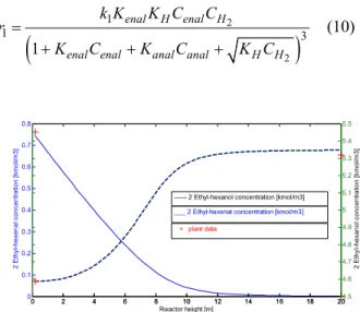
The reaction rates are described by (Smelder, 1989):
2 2
1
1 3
1
enal H enal H
enal enal anal anal H H
k K K C C
r
K C K C K C
(10)
2 2
2
2 3
1
anal H anal H
enal enal anal anal H H
k K K C C
r
K C K C K C
(11)
where Ki is the adsorption equilibrium constant for
component i (i: enal, anal, H), Ci concentration of
component i and ki rate constant of surface reaction
i,(i:1,2).
The rate of reaction incorporating the catalyst de-activation can be obtained as follows:
, ( )
i d i
r r a t (12)
where: a is a fraction of active catalyst and ri is the
reaction rate of species i.
For validation of the developed model a con-siderable number of trials were chosen to compare simulation results with plant data (NIST, 2011;
Gas-par et al., 2010; Perry et al., 1999; Tobiensen et al.,
2008, Silva et al., 2003) and the two most repre-sentative cases are presented in Table 1, which em-phasizes the small differences between the plant data and simulated values.
Table 1: Data validation.
Run H2
concentration (kmol/m3
)
2-ethyl-hexenal concentration
(kmol/m3
)
2-ethyl-hexanol concentration
(kmol/m3
)
Outlet liquid temperature
(K) sim plant sim plant sim plant sim plant
1 0.078 0.0549 0.0021 0.0020 5.346 5.32 441.6 441.3 2 0.088 0.055 0.0022 0.0023 5.343 5.31 442.1 441.5
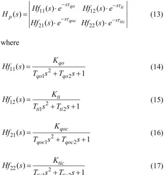
The accuracy of the distributed parameter nonlinear mathematical model of the process is highlighted by the evolutions of 2-ethyl-hexenal, 2-ethyl-hexanol con-centrations and the temperature evolution along the reactor height, presented in Figure 2 and Figure 3.
Figure 2: 2-ethyl-hexenal and 2-ethyl-hexanol concentration profile along the reactor height - RUN 1.
Figure 3: Outlet liquid temperature profile along the reactor height - RUN 1.
0 2 4 6 8 10 12 14 16 18 20
0 0.1 0.2 0.3 0.4 0.5 0.6 0.7 0.8
Reactor height [m]
2
E
th
yl
-h
e
xe
n
a
l
co
n
c
e
n
tr
a
ti
o
n
[
k
m
o
l/
m
3
]
0 2 4 6 8 10 12 14 16 18 204.5
4.6 4.7 4.8 4.9 5 5.1 5.2 5.3 5.4 5.5
2
E
th
yl
-h
e
xa
n
o
l
co
n
c
e
n
tr
a
ti
o
n
[
k
m
o
l/
m
3
]
___ 2 Ethyl-hexenal concentration [kmol/m3] --- 2 Ethyl-hexanol concentration [kmol/m3]
+ plant data
0 2 4 6 8 10 12 14 16 18 20
370 380 390 400 410 420 430 440 450
Reactor height [m]
O
u
tl
e
t
liq
u
id
t
e
mp
e
ra
tu
re
[
K
]
__Outlet liquid temperature [K]
Operational Mathematical Model
Due to the fact that nonlinear mathematical models are more accurate, but also too complex for efficient use in controller design, the authors propose another approach, to use a simple operational model of the process which describes its most important proper-ties (Iancu et al., 2010; Simson et al., 2001).
The linear operational mathematical model was determined using experimental identification methods based on plant data, as a transfer function matrix of second order elements between the main input and output variables (Both, 2012): the 2-ethyl-hexanol recirculated flow (Qoct), the input temperature of the reactants (Tin), the output temperature of the product (Tout) and the output concentration of the product (Cout).
11 12
21 22
( ) ( )
( )
( ) ( )
qo ti
qoc tic
s s
p s
s
Hf s e Hf s e
H s
Hf s e Hf s e
(13)
where
11 2
1 2
( )
1
qo
qo qo
K
Hf s
T s T s (14)
12 2
1 2
( )
1
ti
ti ti
K
Hf s
T s T s (15)
21 2
1 2
( )
1
qoc
qoc qoc
K
Hf s
T s T s (16)
22 2
1 2
( )
1
tic
tic tic
K
Hf s
T s T s (17)
The input hydrogen pressure (P) and 2-ethyl-hex-enal flow (Qenal) act as disturbances. The transfer matrix describing the dependence between the output variables and the disturbances is:
11 12
21 22
( ) ( )
( )
( ) ( )
qe p
qec pc
s s
dist dist
dist s s
dist dist
Hf s e Hf s e
H s
Hf s e Hf s e
(18)
where
11 2
1 2
( )
1
qe dist
qe qe
K
Hf s
T s T s (19)
12 2
1 2
( )
1
p dist
p p
K
Hf s
T s T s (20)
21 2
1 2
( )
1
qec dist
qec qec
K
Hf s
T s T s (21)
22 2
1 2
( )
1
pc dist
p c p c
K
Hf s
T s T s (22)
Following the previous equations, the transfer matrix of the simplified hydrogenation reactor is:
( ) ( )
p dist
Tout Qoct Qenal
H s H s
Coct Tin P (23)
Using the operational mathematical model, the plant data and the simulation results of the nonlinear validated mathematical model, analysis of the dynamical behavior of the simplified model is done. Figure 4 and Figure 5 present the evolution of the output temperature (Tout) for a +14% step variation of the 2-ethyl-hexenal input flow and for a step variation in the 2-ethyl-hexanol recirculated flow.
Figure 4: Outlet liquid temperature evolution: change
in Qenal.
Figure 5: Outlet liquid temperature evolution: change in Qoct.
2600 2800 3000 3200 3400 3600 3800 4000 440
442 444 446 448 450 452 454
Time [s]
Tout [K]
nonlinear model simplified model
2600 2800 3000 3200 3400 3600 3800 4000 424
426 428 430 432 434 436 438 440 442 444
Time [s]
Tout [K]
160 Roxana Both, Eva-Henrietta Dulf and Ana-Maria Cormos
The validation of the simplified linear mathemati-cal model is based on the comparison between equa-tion results and plant data. The presence of an ac-ceptable error is emphasized in the previous figures.
RELATIVE GAIN ARRAY (RGA) ANALYSIS
Considerable research effort was dedicated to the development of control techniques for MIMO pro-cesses, but it still represents a difficult task in practi-cal engineering. At the present time, there are two main directions of approach in control design for multivariable processes. The first approach supports the idea to design a centralized MIMO controller, which implies the use of algebraic decoupling methods or optimal control theory. However, the result is a complex controller, difficult to implement. Another approach is to design a decentralized controller, which attempts to control a fairly multivariable pro-cess by separating the control problem into several SISO (single – input, single - output) systems and then uses conventional control for each loop. The advantages of this approach are very clear: simple to design, easy to implement or tune (fewer parameters); hence it is more often used in practical applications. However, the main disadvantage is represented by the substandard closed loop performance due to in-teractions between loops. A mandatory step is to determine the appropriate loop configuration in order to obtain minimal interactions between loops. This is achieved by proper pairing of the manipulated and controlled variables. In the chemical industry the process complexity reaches up to several hundred control loops, making input – output pairing a diffi-cult task. This task is also essential because it can lead to an unstable overall system, even if the indi-vidual loops are stable.
In 1996, Bristol (1966) introduced the Relative Gain Array technique to determine a measure of the process interactions, giving advice in solving the pairing problem. This technique considers only the steady-state gains of the process to determine the best pairing solution. Due to its simplicity, the RGA technique was widely used in different applications and still has the widest application in industry. The main disadvantage of this technique is represented by the lack of dynamic information of the process, which may sometimes lead to an incorrect loop pair-ing decision. A dynamic version of the RGA tech-nique was developed by McAvoy (1983). The dy-namic RGA (DRGA), in comparison with the RGA, uses the transfer function model instead of the steady-state gain matrix in order to consider the process
dynamics, giving a more accurate interaction assess-ment. Xiong (2005) combined in his work the ad-vantages of both RGA and DRGA by introducing the concept of an effective relative gain array (ERGA), which provides an accurate, detailed and easy to understand description of the dynamic interaction among individual loops without the need to specify the controller type.
In this study the RGA technique was used to de-termine the best control loop pairs and, at the end, the performances of the selected control loop pairs are studied. RGA is represented by a matrix with one column for each input variable and one row for each output variable. From this matrix one can easily com-pare the relative gains associated with each input-output variable pair and match the input and input-output variables that have the biggest effect on each other, while also minimizing undesired side effects. Standard analysis suggests that RGA elements corresponding to input-output pairings close to 1 should be pre-ferred. Negative or large RGA elements are disad-vantageous as they correspond to loops which may be nominally stable, but which become unstable if saturation occurs (e.g. (Bristol, 1966)).
The simplest approach was found to be the use of the developed linear mathematical model and and to compute RGA from the steady-state gain matrix. The steady-state gain matrix is thus obtained with its elements:
qo ti
qoc tic
K K
Tout Qoct
Coct K K Tin (24)
The RGA, for a non-singular square matrix G, is a square complex matrix defined as RGA G( ) G G( 1) ,T
where x denotes element-by element multiplication (Hadamard or Schur product).
For the obtained steady-state gain matrix Hp0
0
2.1 0.0049
1 0.011
Tout Coct
p
Qoct H
Tin (25)
and
0
1.2692 0.2692
( )
0.2692 1.2692
Tout Coct
p
Qoct RGA H
Tin (26)
From the RGA matrix one can observe that there is a strong coupling between Qoct and Tout and Tin
MULTIVARIABLE SMITH PREDICTOR PID CONTROLLER DESIGN
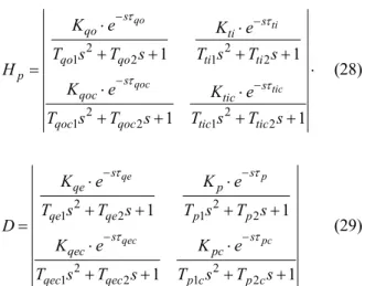
The previously presented linear simplified opera-tional mathematical model of the hydrogenation process consisting of a transfer matrix Hp, which describes the influence of the control inputs u on the controlled outputs y (Tout, Cout), and a transfer ma-trix Hdist, describing the effect of disturbances in the feed z (the input 2-ethyl-hexenal flow Qenal, hydro-gen pressure P) on the outputs y is used in order to develop a multivariable PID controller.
p
y H u D z (27)
Both matrices Hp and D are (2,2)-matrices.
2 2
1 2 1 2
2 2
1 2 1 2
1 1
1 1
qo ti
qoc tic
s s
qo ti
qo qo ti ti
p s
s
qoc tic
qoc qoc tic tic
K e K e
T s T s T s T s
H
K e K e
T s T s T s T s
(28)
2 2
1 2 1 2
2 2
1 2 1 2
1 1
1 1
qe p
qec pc
s s
qe p
qe qe p p
s s
qec pc
qec qec p c p c
K e K e
T s T s T s T s
D
K e K e
T s T s T s T s
(29)
The hydrogenation process is characterized by the presence of time delays. A typical approach to deal with time delay is the non-delayed output prediction (Melo, 2008; Wang, 2008). The non-delayed output may be estimated and the controller can be computed as for a process without delay. The most popular output predictor is the Smith Predictor, Figure 6.
C sT
f P H e
H
Hf esT
ysp
+ -
- +
+
+ + +
y d
Figure 6: Smith predictor structure.
For the controller design the transfer matrix of the process without disturbance is used:
2 2
1 2 1 2
2 2
1 2 1 2
11 12
21 22
1 1
( )
1 1
( ) ( )
( ) ( )
qo ti
qoc tic
qo ti
qoc tic
s s
qo ti
qo qo ti ti
p s
s
qoc tic
qoc qoc tic tic
s s
s s
K e K e
T s T s T s T s
H s
K e K e
T s T s T s T s
Hf s e Hf s e
Hf s e Hf s e
(30)
The desired multivariable controller matrix has the following form [34]:
11 12
21 22
( ) ( )
( )
( ) ( )
R
HR s HR s
H s
HR s HR s (31)
where HR11, HR22 are designed for the direct control of the outputs and HR12, HR21are designed to com-pensate the coupling effect.
Considering the large time delays of the plant the Smith Predictor structure is used, presented in Figure 7.
HR11 Hf11 esT ref1
-
+
+
y1 d1
ref2
HR21
HR12
HR22
Hf21
Hf12
Hf22
sT
e
sT
e
sT
e
Hf11 esT
Hf21
Hf12
Hf22
sT
e
sT
e
sT
e d2
y2
-
-
-
Figure 7: Closed loop control scheme using the Smith predictor structure.
All the controllers are computed using the imposed phase margin design method, for k*60 .
162 Roxana Both, Eva-Henrietta Dulf and Ana-Maria Cormos
11
12
21
22
1
( ) 1.3259 1 ;
102.3018
1
( ) 2.7733 1 ;
106.6667
1
( ) 595.6621 1 ;
90.4977
1
( ) 223.8721 1 ;
119.0476
HR s
s
HR s
s
HR s
s
HR s
s
(32)
INTERNAL MODEL CONTROL DESIGN
As presented before, the most popular structure for time delay compensation is the Smith Predictor struc-ture. A very important step in the multivariable Smith Predictor structure is the decoupling of the process. A modified multivariable Smith Predictor structure was proposed by Wang, Zou and Zhang (Wang et al., 2000). In this case the decoupling matrix is com-puted in frequency domain. More recently the Internal Model Control (IMC) method was used in order to compute the decoupling matrix (Wang et al., 2002). Chen et al. (2011) used the IMC method only as an intermediary step in order to compute the final con-troller – a matrix of PI concon-trollers. The method used in this paper is based on the approach proposed by
Pop et al. (2011) in which the IMC controllers are
used as final controllers.
The model of the process is assumed to be equal to the process transfer function matrix Hp, presented before:
11 12
21 22
( ) ( )
( )
( ) ( )
qo ti
qoc tic
s s
m m
m s
s
m m
Hf s e Hf s e
H s
Hf s e Hf s e
(33)
The next steps in order to design the IMC control-lers are: a) Determine the pseudo-inverse matrix; b) Determine the decoupled process; c) Approximate the elements on the first diagonal of the steady-state de-coupled process matrix; d) Design the IMC controllers.
The method used to decouple the multivariable system is the pseudo-inverse (Skogestad, 2011) of the steady state gain matrix:
11 0 12 0
21 0 22 0
(0) m m
m
m m
Hf Hf
H
Hf Hf (34)
The pseudo-inverse is computed based on the fol-lowing equation (Skogestad, 2011):
# 1
(0) ( (0) (0) )
H H
m m m m
H H H H (35)
where Hm# is the pseudo-inverse which will act as a pre-compensator matrix.
The decoupled multivariable process is done by:
11 12
#
21 22
( ) ( ) d d
D m m
d d
Hf Hf
H s H s H
Hf Hf (36)
The matrix (36) represents the steady-state decou-pled process, in which all elements are weighted sums of the original transfer functions Hfijes. Due to
the static decoupling, the steady-state matrix ( )0
D
H s will be equal to the unit matrix. In this way all the elements which are not on the first diago-nal will be equal to zero.
The next step is to approximate the elements on the first diagonal of the matrix HD( )s with simple transfer functions:
*
( ) ( )
iid iid
Hf s Hf s (37)
The elements on the first diagonal, approximated by the transfer function given in (37), will be used for controller design.
The approximation of each element Hfiid*( )s can be obtained by using genetic algorithms or graphical identification methods (Chen et al., 2011).
The next step is to design the IMC controller as follows (Chen et al., 2011):
*
( ) ( ) ( )
IMCi iid inv
HR s Hf s f s (38)
where f s( ) is the IMC filter and Hfiid inv *( )s repre-sents the invertible part of Hfiid*( )s . The IMC filter is computed as:
1 ( )
( 1)
n
i
f s s
(39)
where λi is the time constant of the filter associated
o st H H u M co an th tr fu F co vershoot, th tudy results i
1 2 100 4 20 1 IMC IMC HR HR Figure Figure Figure 10 sing delay Moore-Penros ompensator f
nd the fast m he time delay
rix of all elem unction matri
Figure 10: C ontrollers. 1000 440 442 444 446 448 450 452 Tout [K] 1000 5.35 5.4 5.45 5.5 5.55 5.6 5.65 Coct [Kmol/m 3]
he final IMC in the follow
2 2 2 2 00 55.85 400 40 0001 87.2 100 20 s s s s s s
8: Tuning of
9: Tuning of
presents the compensator se pseudo-inv for the proces
model Hm( )s
ys). HD*
sments Hfiid*(
ix HD*( )s w
Closed loop 1500 T 1500 T C controller wing transfer 1 and 1 2 1 1 s s
f the controll
f the controll
closed loop r and IMC verse Hm# is ss Hp( )s , the
)(the process is the transf
( )s and H*D(s
without the tim
control sche 2000 250 Time [s]
2000 250 Time [s]
rs for the c function:
(4
ler IMC1.
ler IMC2. control sche controller. T s used as a p
e model Hm
s model with fer function m
)
s is the trans me delay.
eme using IM 500 3000 λ=5 λ=10 λ=15 λ=20 500 3000 λ=5 λ=10 λ=15 λ=20 case 40) eme The
pre-( )s
hout ma-sfer MC im Gu in con sce tur bo ba sar con Th sce the con the con ou enc tem Fig var Fig for 0.2 0 0 Coct [Kmol/m 3] SI For analysis mplemented i uide, 2008). T
comparison nclude the re enarios are t rbance reject th control st sed on the li ry to test th nsidering th his analysis
enario. The first sim e set-point tr
ntrol strategi To this end e output tem nsidered. Fig utput tempera
ce of the re mperature on
gure 11: Ou riation on inp
gure 12: 2-E r a step varia
For the sam 25 [kmol/m3] 0 1000 440 442 444 446 448 450 452 Tout [K] 0 1000 5.29 5.3 5.31 5.32 5.33 5.34 5.35 5.36 Coct [Kmol/m 3] IMULATIO
s purposes b in Matlab/S The simulati for the two c esults. The t the set-point tion analysis trategies, the inear model he robustness he variation is performe mulation sce racking perf ies. a reference mperature of gure 11 pres ature while F eference step n the
2-ethyl-utput temper put 1.
Ethyl-hexano ation on inpu
me analysis a ] is consider 00 2000 30
Tim
00 2000 30 Tim
ON RESULT
oth control s SIMULINK
ion scenarios control strateg two main obj tracking ana s. Due to the controllers w of the proce s of the con of the mode ed in the thi
enario is focu formances of
step variatio f the produc sents the ev Figure 12 sh p variation f -hexanol con
rature evolut
ol concentra ut 1.
reference ste red for the 2-3000 4000 Time [s] IMC PID 3000 4000 ime [s] IM P TS structures we (Matlab Us s are presente
gies in order jectives of th alysis and di e fact that, f were designe ess, it is nece ntrol strategi el parameter ird simulatio
used on testin f the designe
on of 10 K f ct at t=10s volution of th hows the infl
for the outp ncentration.
tion for a ste
164 Roxana Both, Eva-Henrietta Dulf and Ana-Maria Cormos
output concentration. The evolution of the 2-ethyl-hexanol concentration is presented in Figure 13. and the influence of the reference step variation on the output temperature is detailed in Figure 14.
To reach the second objective of the section, the second simulation scenario is focused on the disturb-ance rejection analysis of the designed control strate-gies. Figure 15 and Figure 16 present the effects of a 0.25 [kmol/m3] disturbance in 2-ethyl-hexenal flow on the two considered outputs.
Figure 13: Output temperature evolution for a step variation on input 2.
Figure 14: 2-Ethyl-hexanol concentration evolution for a step variation on input 2.
Figure 15: Output temperature evolution for a dis-turbance in 2-ethyl-hexenal flow.
Figure 16: 2-Ethyl-hexanol concentration evolution for a disturbance in 2-ethyl-hexenal flow.
From all the above figures it can be concluded that the IMC control strategy presents better perfor-mances in comparison with the MIMO PID control. Another advantage of the method is that it is more straightforward and easy to design. The minor disad-vantage is the Lag-Lead form of the controllers op-posite to the classical PID forms.
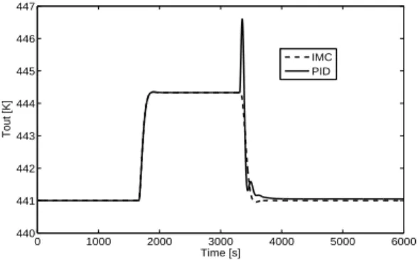
The last objective of this section is to test the ro-bustness of the designed control strategies. To this end, the following figures present the evolution of the output temperature and 2-ethyl-hexanol concen-tration considering a reference step variation for both variables and also the variation of the uncertain pa-rameters of the linear plant.
The closed loop simulations using the multivaria-ble Smith Predictor PI controller under nominal pa-rameter values (solid black line), as well as the simu-lations considering the variation of the uncertain parameters of the linear plant (solid grey lines), for a reference step variation of the output temperature are presented in Figure 17 and Figure 18. The uncertain parameters considered are the time constants of the process as well as the gain parameter.
Figure 17: Output temperature evolution for a step variation on input 1– nominal case vs. uncertain case (PID).
0 1000 2000 3000 4000 5000 6000 438
440 442 444 446 448 450 452
Time [s]
Tout [K]
IMC PID
0 1000 2000 3000 4000 5000 6000 5.35
5.4 5.45 5.5 5.55 5.6 5.65
Time [s]
Coct [Kmol/m
3]
IMC PID
0 1000 2000 3000 4000 5000 6000 440
441 442 443 444 445 446 447
Time [s]
Tout [K]
IMC PID
0 1000 2000 3000 4000 5000 6000 5.3
5.31 5.32 5.33 5.34 5.35 5.36 5.37 5.38 5.39 5.4
Time [s]
Coct [Kmol/m
3]
IMC PID
1000 2000 3000 4000 5000 6000 440
442 444 446 448 450 452 454
Time [s]
Figure 18: 2-Ethyl-hexanol concentration evolution for a step variation on input 1– nominal case vs. un-certain case (PID).
The closed loop simulations using the multivaria-ble Smith Predictor PI controller under nominal pa-rameter values (solid black line), as well as the simu-lations considering the variation of the uncertain parameters of the linear plant (solid grey lines), for a reference step variation of the 2-ethyl-hexanol con-centration are presented in Figure 19 and Figure 20.
Figure 19: Output temperature evolution for a step variation on input 2– nominal case vs. uncertain case (PID).
Figure 20: 2-Ethyl-hexanol concentration evolution for a step variation on input 2– nominal case vs. un-certain case (PID).
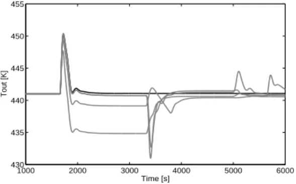
In order to choose the control algorithm with the best performances, the same simulation scenario is considered for the IMC controller. To this end, the closed loop simulations using the IMC controller in Smith Predictor structure under nominal parameter values (solid black line), as well as the simulations considering the variation of the uncertain parameters of the linear plant (solid grey lines), for a reference step variation of the output temperature are presented in Figure 21 and Figure 22.
Figure 21: Output temperature evolution for a step variation on input 1– nominal case vs. uncertain case (IMC).
Figure 22: 2-Ethyl-hexanol concentration evolution for a step variation on input 1– nominal case vs. un-certain case (IMC).
The closed loop simulations using the IMC con-troller in Smith Predictor structure under nominal parameter values (solid black line), as well as the simulations considering the variation of the uncertain parameters of the linear plant (solid grey lines), for a reference step variation of the 2-ethyl-hexanol con-centration are presented in Figure 23 and Figure 24.
Based on the simulation results presented, it can be concluded that the most appropriate control egy with satisfactory results is the IMC control strat-egy in Smith Predictor structure.
It can be observed that the differences between the performances of the nominal and perturbed sys-1000 2000 3000 4000 5000 6000
5.2 5.25 5.3 5.35 5.4 5.45
Time [s]
Coct [Kmol/m
3]
1000 2000 3000 4000 5000 6000 430
435 440 445 450 455
Time [s]
Tout [K]
1000 2000 3000 4000 5000 6000 5.4
5.5 5.6 5.7 5.8 5.9 6 6.1
Time [s]
Coct [Kmol/m
3]
1000 2000 3000 4000 5000 6000 440
442 444 446 448 450 452 454
Time [s]
Tout [K]
1000 2000 3000 4000 5000 6000 5.3
5.31 5.32 5.33 5.34 5.35 5.36 5.37
Time [s]
Coct [Kmol/m
166 Roxana Both, Eva-Henrietta Dulf and Ana-Maria Cormos
tems are smaller than in the case of classical control, Figure 17 to Figure 24. It must be mentioned that the simulation scenarios are considered for four extreme points of operation, implying a very large range of parameter variation. If the variation range of the uncertain parameters is smaller, in normal operation conditions, the differences between the performances of the nominal and perturbed systems are very small.
Figure 23: Output temperature evolution for a step variation on input 2– nominal case vs. uncertain case (IMC).
Figure 24: 2-ethyl-hexanol concentration evolution for a step variation on input 2– nominal case vs. un-certain case (IMC).
CONCLUSIONS
This paper describes the two control strategies of an important chemical process, the 2-ethyl-hexenal hydrogenation process, in a catalytic fixed-bed reac-tor. This process is a nonlinear system with dis-tributed parameters. However, it is possible to de-scribe the processes that occur inside the reactor by a linear nominal transfer matrix.
Several simulation scenarios are considered in or-der to choose the control algorithm with the appro-priate performances. The simulation results pre-sented in the sixth section of the paper show that the
IMC control presents better performances for set-point tracking and also for disturbance rejection tests, and better robustness, so it is recommended for implementation. Additionally, this method reduces the design burden of the controllers.
NOMENCLATURE
Ci molar concentration (kmol/m3) cpi specific heat capacity (kJ/kmol K) F volumetric flow rate (m3/s)
T Temperature (K)
ΔRH reaction heat (kJ/kmol)
K adsorption equilibrium constant, component i (m3/mol)
k rate constant of surface reaction j (mol/s kg) HH2 Henry’s law constant
v velocity (m/s)
S reactor cross-sectional area (m2) M molecular mass (kg/kmol)
av specific gas-liquid contact area (m-1) r rate of surface reaction (mol/s kg)
t time (s)
z axial reactor coordinate
Greek Letters
ρ density (kg/m3)
Subscripts/Superscripts
G gas phase
L liquid phase
i H2, 2-ethyl-hexenal, 2-ethyl-hexanal, 2-ethyl-hexanol
j 2-ethyl-hexenal hydrogenation reaction, 2-ethyl-hexanal hydrogenation reactor
ACKNOWLEDGEMENTS
This work was supported by a grant of the Roma-nian National Authority for Scientific Research, CNDI– UEFISCDI, project number 155/2012 PN-II-PT-PCCA-2011-3.2-0591.
REFERENCES
Attou, A., Boyer, C., Ferschneider, G., Modeling of hydrodynamics of the cocurrent gas-liquid trickle flow in a trickle-bed reactor. Chemical Engineer-ing Science, 54, 785-802 (1999).
0 1000 2000 3000 4000 5000 6000 420
425 430 435 440 445
Time [s]
Tout [K]
10005 2000 3000 4000 5000 6000 5.2
5.4 5.6 5.8 6 6.2
Time [s]
Coct[Kmol/m
Both, R., Eva-Henrietta Dulf, Clement Feştilă, Ro-bust control of a catalytic 2-ethyl-hexenal hydro-genation reactor. Journal of Chemical Engineering Science, ISI, (2012). doi: 10.1016/j.ces.2012.02. 033.
Both, R., Ana Maria Cormoş, Paul Şerban Agachi, Clement Feştilă, Dynamic modeling and valida-tion of the 2-ethyl-hexenal hydrogenavalida-tion process. Computer & Chemical Engineering, 52, 100-111 (2013). http://dx.doi.org/10.1016/j.compchemeng. 2012.11.012
Bozga, G., Muntean, O., Chemical reactors. Bucur-esti, Technique Editure, v. 2, Chapter 6 (2001). (In Romanian).
Bristol, E. H., On a new measure of interactions for multivariable process control. IEEE Transactions on Automatic Control, 133-134, 11:1 (1966). Burghardt, A., Grazyna, B., Miczylaw, J., Kolodziej,
A., Hydrodynamics and mass transfer in a three-phase fixed bed reactor with cocurrent gas-liquid downflow. The Chemical Engineering Journal, 28, 83-99 (1995).
Chen, J., He, Z.-F. Qi, X., A new control method for MIMO first order time delay non-square systems. Journal of Process Control, 21(4), 538-546 (2011).
Collins, D. J., Grimes, D. E., Davis, B. H., Kinetics of the catalytic hydrogenation 2-ethyl- hexenal. The Canadian Journal of Chemical Engineering, 61, 36-39 (2009).
Coker, K., Modeling of Chemical Kinetic and Reac-tor Design. Gulf Publishind Company, Chapters 2, 3, 4, 6 (2001).
Gaspar, J., Cormos, A. M., Dynamic modeling and validation of absorber and desorber columns for post-combustion CO2 capture. Computers and Chemical Engineering, 35(10), 2044-2052, (2010). doi:10.1016/j.compchemeng.2010.10.001 Iancu, M., Agachi, S., Optimal process control of an
industrial heat integrated fluid catalytic cracking plant using model predictive control. 20th Euro-pean Symposium on Computer Aided Process En-gineering ESCAPE (2010).
ICIS, <http://www.icis.com/> (Accessed: April 04, 2011).
Iliuta, I., Thyrion, F. C., Bolle, L., Giot, M., Com-parison of hydrodynamic parameters for counter-current and cocounter-current flow through packed beds. Chemical Engineering Science, 20, 171-181 (1997).
Kvamsdal, H. M., Jakobsen, J. P., Hoff, K. A., Dy-namic modeling and simulation of a CO2 absorber column for postcombustion CO2 capture. Chemi-cal Engineering Process, 48, 135-144 (2009).
Lawal, A., Wang, M., Stephenson, P., Koumpouras, G., Yeung, H., Dynamic modeling and analysis of post-combustion CO2 chemical adsorption pro-cess for coal-fired power plants. Fuel, 89, 2791-2801 (2010).
McAvoy, T. J., Some results on dynamic interaction analysis of complex control systems. Ind. Eng. Chem. Process Des. Dev., 22, 42 (1983).
Mahmud, M., Faizi, A. K., Anchoori, V., Al-Qahtani, A., Liquid phase catalytic hydrogenation process to convert aldehydes to the corresponding alco-hols. Patent No. US 6600078 B1 (2003).
MATLAB Users Guide. The MathWorks Inc (2008). Mattos, A. R. J. M., Probst, S. H., Afonso, J. C.,
Schmal, M., Hydrogenation of 2-ethyl-hexen-2-al on Ni/Al2O3 Catalyst. Journal of Brazilian Chemi-cal Society, 15, 760-766 (2004).
Melo, D. N. C., Costa, C. B. B., Toledo, E. C. V., Santos, M. M., Maciel, M. R. W., Maciel Filho. R., Evaluation of control algorithms for three phase hydrogenation catalytic reactors. Chemical Engineering Journal, 141, 250-263 (2008).
National Institute of Standards and Technology, <http://www.nist.gov/> (Accessed: April 04, 2011). Niklasson, C., Kinetics of adsorption and reaction for
consecutive hydrogenation of 2-ethylhexenal on Ni/SiO2 catalyst. Industrial & Engineering Chemis-try Research, 26, 403-410 (1987).
Niklasson, C., Kinetics of hydrogenation of 2-ethyl-hexenal and hydrogen/deuterium exchange on a palladium/silica catalyst in a continuously stirred tank reactor. Industrial & Engineering Chemistry Research, 27(11), 1990-1995 (1988).
Olah, G. A., Molnar, A., Hydrocarbon Chemistry. 2nd Ed., New York, John Wiley & Sons, Chapter 11 (2003).
Pavlov, C. F., Romankov, P. G., Processes and Ap-paratus in Chemical Engineering. Bucuresti, Tech-nique Editure (1981). (In Romanian).
Perry, R. H., Green, D. W., Perry’s Chemical Engi-neers’ Handbook. 8th Ed., New York, McGraw-Hill (1999).
Pop, C. I., De Keyser, R., Ionescu. C., A simplified control method for multivariable stable nonsquare systems with multiple time delays. Control & Au-tomation (MED), 19th Mediterranean Conference, Proceedings, 382-387 (2011). doi: 10.1109/MED. 2011.5983051.
Silva, J. D, Lima, F. R. A., Abreu, C. A. M., Knoechelmann, A., Experimental analysis and evaluation of the mass transfer process in a trickle-bed reactor. Brazilian Journal of Chemical Engineering, 20, 375-390 (2003).
168 Roxana Both, Eva-Henrietta Dulf and Ana-Maria Cormos
J. K., Metamodels for computer-based engineering design: Survey and recommendations. Engineering with Computers, 17(2), 129-150 (2001).
Skogestad, S., Postlethwaite, I., Multivariable Feed-back Control: Analysis and Design. New York, John Wiley & Sons (2005).
Smelder, G., Kinetic Analysis of the liquid phase hydrogenation of 2-ethyl-hexenal in the presence of supported Ni,Pd and Ni-S catalyst. The Canadian Journal of Chemical Engineering, 67, 51-61 (1989). SRI Consulting, IHS Inc, < http://www.sriconsulting.
com/> (Accessed: March 07, 2011).
Tobiesen, F. A., Juliussen, O., Svendsen, H. F., Ex-perimental validation of a rigorous desorber model for CO2 postcombustion capture. Chemical Engineering Science, 63, 2641-2656 (2008).
Wang, Q. G., Ye, Z., Cai, W-J., Hang, C-C., PID Control for Multivariable Processes. Springer-Verlag Berlin Heidelberg (2008).
Wang, Q. G., Zou, B., Zhang, Y., Decoupling Smith predictor design for multivariable systems with multiple time delays. Chemical Engineering Re-search and Design, 78, 565-572 (2000).
Wang, Q. G., Zhang, Y., M. Chiu, S., Decoupling internal model control for multivariable systems with multiple time delays. Chemical Engineering Science, 57, 115-124 (2002).
World Resources Institute, <http://www.wri.org/> (Accessed: November 23, 2009).