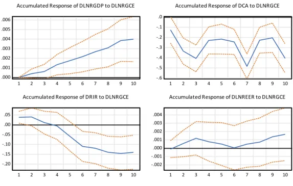
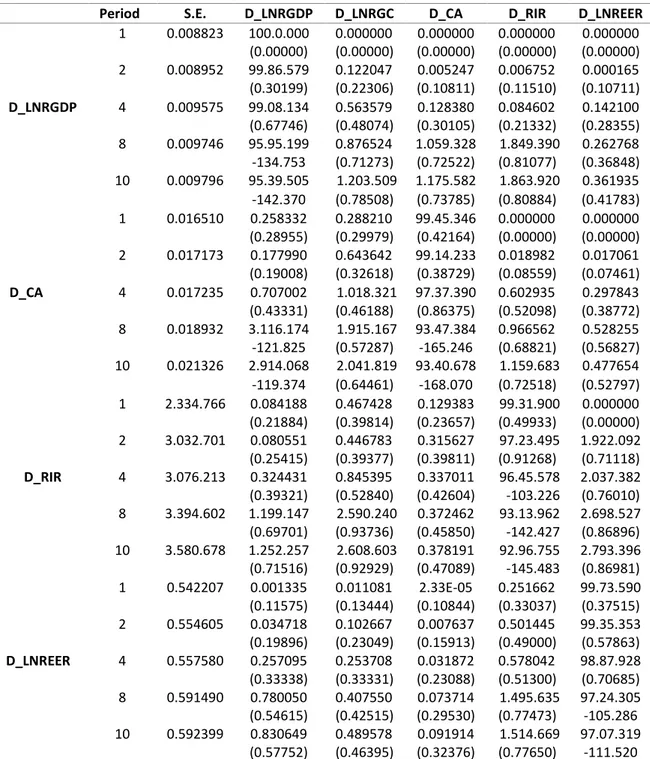
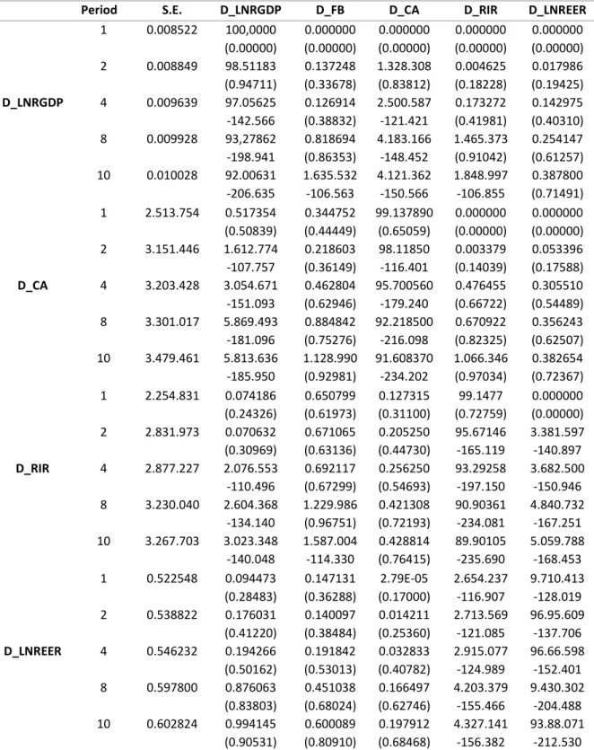
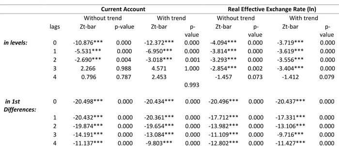
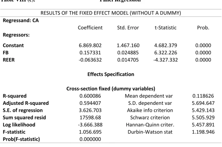
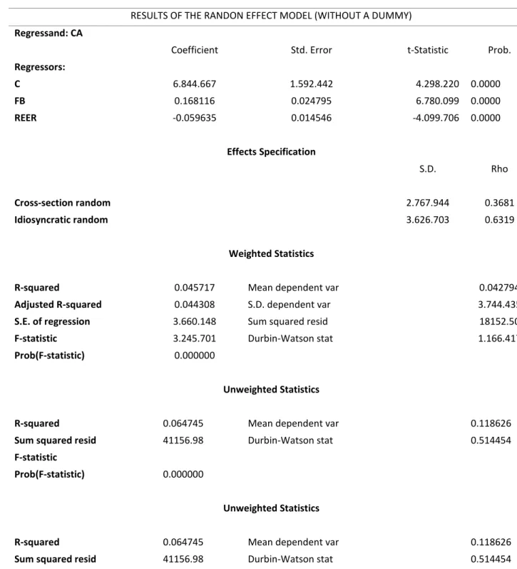
The linkages between fiscal and current account imbalances
53
0
0
Texto
Imagem
+7
Documentos relacionados