Servicing the public debt : the role of government’s behavior towards debt

(1)

Universidade Católica Portuguesa

Master’s Thesis

Servicing the Public Debt: the Role of

Government’s Behavior Towards Debt

Candidate:

Ricardo Oliveira Alves Monteiro

152212007

Supervisor:

Professor Pedro Teles

Dissertation submitted in partial fulfillment of requirements for the degree of MSc in Economics, at Universidade Católica Portuguesa, September 2014.

(2)

Servicing the Public Debt: the Role of

Government’s Behavior Towards Debt

Ricardo Monteiro

⇤

September 15, 2014

Supervisor: Pedro Teles

Abstract

This article presents a model in which haircuts on public debt may occur. My focus relies on the explanation and numerical exploration of multiple equilibria. Calvo (1988) first found multiple equilibrium interest rates due to investors’ self-fulfilling expectations of a partial default in a model with exogenous debt. I use Calvo’s (1988) setting to study the impact of endo-genizing debt on multiplicity. This is a relevant exercise as in this setting the government has the ability to choose the optimal level of debt. More than that, if it behaves as a large agent it can influence the interest rate it will face. In particular, I find that if the interest rate schedule is presented as in Arellano (2008), depending on debt at maturity, uniqueness can be achieved by a government behaving as a large agent. However, investors can also coordinate on oﬀering a schedule depending on the initial level of debt, as implicitly defined in Calvo (1988). In this case there is more than one equilibrium, provided that public expenditure in the first period is not extremely high.

(3)

(4)

Acknowledgments

I am very grateful to my supervisor, Professor Pedro Teles, for his guidance and advice throughout the MSc, particularly during the process of writing this dis-sertation. I would also like to thank Professors Catarina Reis, Leonor Modesto, Miguel Gouveia and Pedro Raposo for their time and comments and to Professor Teresa Lloyd-Braga for always being there, ready to help, with a smile on her face. Furthermore, I want to thank Católica-Lisbon not only for the opportunity of learning Economics, but also for teaching undergraduate students from which I also learned a lot.

I want to thank all my friends that supported me until here and during this process. A special mention needs to be done to my friends on the teaching assis-tants’ room (especially Eduardo Catroga, Joana Garcia, João Almeida and Jordi Martins) for listening me going on about schedules, repudiation and equilibrium conditions, and for all the (more than academic) support not only during the process of writing this dissertation but during the whole MSc program. Apart from my friends at Católica, I also want to thank, in particular, Joana Vicente for the long days of work at her place, since without them and her support I would still be writing this thesis. I also want to acknowledge Sofia for her unconditional support, not only now, but since we met, and for years to come.

Finally, I want to thank my family for supporting me in my choices, backing me up in the hard decisions and making this thesis and all my education possible.

(5)

List of Figures

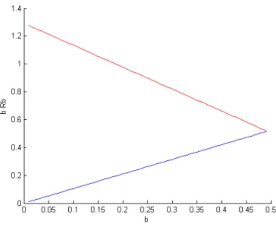
1 Government response function and multiple equilibria . . . 8 2 Interest Rate Schedules for b and bRb . . . 12

3 Demand for debt and Equilibrium (Competitive) in Calvo’s class of schedules . . . 15 4 Demand for debt and Equilibrium (Competitive) in Arellano’s class

of schedules . . . 16 5 Equilibrium (Competitive) with small public expenditure in period 0 17 6 Level of debt versus debt at maturity . . . 20 7 Equilibria with high public expenditure in period 0 . . . 22 8 Equilibria with small public expenditure in period 0 . . . 23

List of Tables

1 Large public expenditure in period 0 . . . 14 2 Small public expenditure in period 0 . . . 16

(7)

(8)

1 Introduction

Recently, the topic of debt restructuring has gained more visibility around the developed world. In fact, with the sovereign debt crisis in Europe and particularly in Greece and Portugal, policy discussions included haircuts, repudiation and probabilities of default. During the crisis we have seen interest rates rising, and with it the costs of servicing public debt. In fact, looking at the evolution of secondary market yields on Portuguese and Greek 10 year government bonds, one can see the rapid increase they have experienced: the secondary market yields on Portuguese 10 year government bonds went from around 4% in the beginning of 2010 to around 16% in the beginning of 2012; the same happened to Greek 10 year government bonds going from around 5% to 32% roughly in the same period of time. Both yields seem to be back to pre-crisis levels. However, Greece ended up restructuring part of its own debt. Motivated by these recent events there has been a return to the research topic of sovereign debt and default, with several authors looking back at Calvo (1988).

Calvo (1988) looks at multiplicity in the context of debt haircuts highlight-ing the role of agents’ expectations. He finds that there are multiple equilibrium interest rates and haircuts where investors’ expectations play an important role: interest rates increase when haircuts are expected to be higher, but haircuts must also be higher when interest rates are higher because the burden of debt is also higher. In other words, if investors believe that the government will default on part of its debt, interest rates go up which will only make it more likely that their debt haircut expectations will be fulfilled. Calvo also found some paradoxical or “unreasonable” high interest rate schedules in which the interest rate goes down when outstanding debt goes up. All in all, his conclusion is that depending on in-vestors’ beliefs there is more than one equilibrium interest rate and corresponding haircut.

Before Calvo (1988), Eaton and Gersovitz (1981) also worked on the problem of a government that may default on international debt. They claim that in their model there is only one type of interest rate schedule. This is based on an assumption that arbitrarily restricts the set of solutions as shown by Navarro, Nicolini and Teles (2014). Therefore, until very recently there were contradictory

(9)

results in the literature, with authors believing that Calvo (1988) had strange properties and that Eaton and Gersovitz (1981) were right on uniqueness.

This article looks back at Calvo (1988), focusing on a two period model, with a benevolent government and individual consumers, in which debt is endogenous. The main difference from Calvo (1988) is that here, instead of being an exogenous variable, the amount of debt borrowed is chosen by the government in period zero. Effectively there are two periods whereas in Calvo’s setting there is only one period; period 0 is only there to state that there is some exogenous debt contracted by the government. Furthermore, I will make explicit Calvo’s class of schedules for the interest rate and also different classes of schedules and see whether there is multiplicity of equilibria when the government behaves competitively, taking the interest rate as given, and when the government behaves as a large agent. Endogenizing debt is of great importance in this context. With exogenous debt it is odd to discuss multiplicity as the optimal choice of debt is not considered, nor the fact that the government can influence the interest rate it faces if it behaves as a large agent. In fact, when we take all of this into consideration there are some interesting results, different from Calvo and in accordance with Navarro et. al (2014).

Both Navarro et. al (2014) and Lorenzoni and Werning (2013) also look at a diﬀerent class of schedules, first defined in Arellano (2008). In those, instead of the schedule being Rb(b)depending on b (the level of debt contracted in zero), it is

Rb(bq)depending on bq = bRb (debt promised to be paid at maturity). The class

of schedules the government will face depends on what investors coordinate to oﬀer. Then, for each schedule the benevolent government will do the best it can. If competitive, the government takes the interest rate as given, if behaving as a large agent, the government takes the schedule as given. Lorenzoni and Werning (2013) simplify Calvo’s model such that there is no choice by the government on taxes and haircuts, just a coordination problem of investors. Navarro, et al. (2014) also work with both classes of schedules and both competitive and large governments, discussing the implications of endogenizing debt, which are not covered in Lorenzoni and Werning (2013). However, their model is also diﬀerent from the one I am presenting here. In fact, there is also a simplification in the sense that there are no decisions from the government, other that the choice

(10)

regarding the level of debt. Nonetheless, they also focus on policy making and specific distributions for the probability of default as in their article instead of haircuts, there is full default and so a probability associated with it.

Several authors have used Calvo’s model with diﬀerent purposes. Corsetti and Dedola (2013) also build on Calvo (1988) looking also at more recent literature. In their paper they introduce uncertainty with an endowment varying between two states. Depending on the state they end up being the burden of taxes also varies. If the endowment is high the burden is low and vice-versa. Their main focus is on policy and on the role of the central bank to stop self-fulfilling debt crisis. Thus, they do not discuss the role of endogenizing debt and the impact it has on multiplicity.

Having said this, there is still room in the literature for what is being presented here: an explanation and numerical exploration of multiplicity taking into account endogenous debt, large governments and investors coordinating to oﬀer one of two diﬀerent classes of schedules, under Calvo’s setting.

The structure of this paper is as follows. In Section 2, I start by presenting the environment in a two period model focusing on what is the role of each agent in this economy. In Section 3, I present the results with exogenous debt as a base case. In Section 4, I solve the problem with endogenous debt, considering the case of a competitive government, for illustration purposes, looking at the impact of this in equilibria and multiplicity. In Section 5, I solve the problem using a more reasonable assumption that the government behaves as a large agent also looking at the implications on equilibria and multiplicity. Finally, I conclude by summarizing the main findings.

2 A Two Period Model

The model analyzed throughout the next sections is adapted from Calvo (1988). I will consider two periods, 0 and 1, and two types of agents, the government and identical consumers. This article will not focus on production as it would not add value to the analysis of the role of government’s behavior towards debt on servicing the public debt. Thus, I assume an exogenous endowment.

(11)

and/or debt, such that its budget constraint holds while maximizing social wel-fare taking into account households’ preferences (i.e. maximizing utility for a representative agent).

Households maximize utility through consumption. They decide how much either they lend to the government or invest in the other asset available in this economy. As investors, they present a schedule of interest rates to the government, which nature I discuss further ahead1_.

In this economy there are two types of assets: public debt and an asset for which there is no possibility of default.

In the following subsections I look in more detail to the structure of this economy.

2.1 Government

In period 0, the government borrows b per capita units of output which will yield Rb units of output per unit of debt held, and not repudiated, to consumers in

period 1. The government is also expected to repudiate a fraction of debt ✓, 0  ✓  1. In this sense, in period 0, the government has to fund exogenous government expenditures, g, and to do so, can use both distortionary taxes, x, and debt, b. In period 1, the government has to repay debt plus interest and the costs of debt repudiation2_{, on top of government expenditures for the current}

period. Having said this, the budget constraints of the government are, in period 0 and 1 respectively:

x0 = g0 b (1)

x1 = g1+ bRb(1 ✓) + ↵✓bRb (2)

1_{Here I am looking at domestic held debt, in this sense households are those investing in}

public debt.

(12)

2.2 Households

Household’s have linear preferences, however I will assume a convex cost for taxes (distortion of taxes is convex). This assures that the problem of the government is well defined as it will smooth the distortions into both periods. In this sense, preferences are such that:

U (c0, c1) = c0+ c1 (3)

In the last period consumers’ wealth is all used in consumption as there is no utility from saving as all will end at the end of period 1. In order to get an interior solution, with positive consumption in both periods, the following needs to be verified3_:

uc(0)

uc(1)

= R_{, R =} 1 (4)

In this sense, there is a continuum of solutions for c0 and c1, as long as (4)

holds. In period 0 consumers can both consume or save to consume in period 1. Apart from public debt, households can also save through an asset without possibility of default, which yields a gross constant return R. Given the partial repudiation ✓, in a perfect foresight equilibrium with positive stock of both assets, as there is no uncertainty4_{, consumers must be indiﬀerent between the two types}

of assets. Thus, by arbitrage we have:

(1 ✓)Rb = R (5)

In period 0, households have both the endowment, y0, and return from the

asset without possibility of default that they had when born, k0R. They use it

to consume, c0, pay taxes, x0, lend to the government, b, and invest in the other

available asset, k1, bearing the distortion of taxes, z(x0). In period 1, households,

on top of the endowment, y1,and return on the asset without possibility of default,

k1R, have the return of the public debt, bRb(1 ✓). Again, they use it to consume,

3_{This is marginal rate of substitution equal to the relative price of consumption in both}

periods. As preferences are linear this condition simplifies to a condition on relative prices only.

(13)

c1, and pay taxes, x1, also bearing the distortion of taxes, z(x1). In this context,

the budget constraints of the households are, in period 0 and 1 respectively: y0 + k0R = c0+ x0+ z(x0) + b + k1 (6)

y1+ k1R + bRb(1 ✓) = c1+ x1+ z(x1) (7)

The distortion of taxes z(x) is a strictly convex function of x, satisfying stan-dard Inada-type conditions and such that:

z(0) = z0(0) = 0 (8)

If this distortion was also present in the government budget constraint with a symmetric sign, then taxes would be lump-sum and z(x) would work as a second lump sum tax on top of x. By introducing it only on the budget constraint of the households it can be seen as the distortion that reduces available resources in the economy (i.e. it will also appear in the resources constraint as it is obtained by plugging in the budget constraint of the government on the household’s budget constraint). This was the way distortions arising from taxes were modeled in Calvo (1988).

3 Base Case: Exogenous Debt

In this section, I start by presenting the solution of the problem if debt was exogenous. This works as a base case and also to present the results in Calvo (1988) in a diﬀerent way. This is a starting point for what I present afterwards: a more complex problem with endogenous debt and a large government.

3.1 Problem Definition and Solution

The benevolent government maximizes social welfare. As households’ preferences are known, it can do that by maximizing utility. Here, as debt is exogenous the government only chooses the fraction of debt that is not paid in period 1. In this sense, the government does not directly impact consumption in period 0: x0 is

(14)

exogenous as both g0 and b are exogenous. Thus, in period 1, the government

faces the problem of choosing the fraction of debt repudiated such that utility is maximized and the resources constraint is satisfied. The problem can then be summarized in the following manner:

max✓U (c1) s.t.

y1 = c1 k1R + g1+ ↵✓bRb + z(g1+ bRb(1 ✓) + ↵✓bRb)

(9) To solve it, one only needs to substitute c1 in the utility function for the

re-sources constraint, achieved by putting together the government budget constraint and the households budget constraint, and then take derivatives with respect to ✓.5 This is possible as Rb is also contracted in period 0. The timing will be

dis-cussed in the next section as it is of more importance when endogenous debt is considered.

Taking derivatives one gets to the first-order condition: z0(g1+ bRb(1 ✓) + ↵✓bRb) =

↵

1 ↵ (10)

Knowing that the government budget constraint for period 1 is x1 = g1 +

bRb(1 ✓) + ↵✓bRb, the first order condition above implicitly defines a unique

x⇤

1 > 0, provided (7) and the fact that z00(x) > 0. This does not mean that ✓ is

unique as ✓ will be increasing with Rb, such that x⇤1 is constant. More than that,

✓ is bounded between 0 and 1, meaning that possibly, given b, and for some levels of Rb it can be the case that x⇤1 is not attainable. If this is the case, this means

that either ✓ = 0 or ✓ = 1.

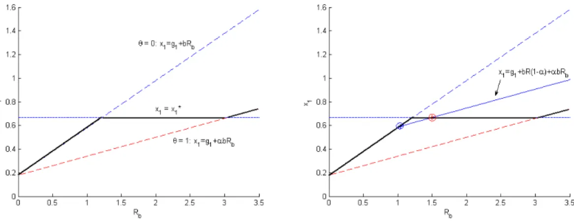
The fraction of repudiation, ✓, is bounded between 0 and 1. A negative ✓ means that the government is repaying more than the promised payment; ✓ > 1 means that the government is not only defaulting on all the contracted debt but also asking investors for more funds. Both scenarios are unreasonable. Thus, replacing the restrictions on ✓ in the budget constraint of the government in period 1 we get a restriction in terms of x1. The government response function

can easily be obtained for this period as in the left panel of Figure 1. To find

(15)

the equilibrium haircuts both (2) and (5) must hold on top of the government response function. In this sense, plugging in (5) in (2) we get the consistency condition depicted in the right panel of Figure 1. It can be seen that, in this case, there are two equilibria with ✓b_(bR

b) and ✓ = 0 being the fractions of debt

repudiated in the bad and good equilibrium, respectively.

Figure 1: Government response function and multiple equilibria

In fact, in Figure 1, one can see two diﬀerent equilibrium interest rates for a given level of debt. In this sense, Calvo stated that there was multiplicity. In the following sections I will use the results of this section, building up on them.

4 The Case of a Competitive Government

After presenting the exogenous case, I solve the problem taking into account the results of the previous section and the setting presented in section 2. I consider a competitive government just for illustration purposes. I understand that this is not the most common assumption as the government is usually seen as being a large agent. However, I am interested in the results for this case, to better understand the problem. Afterwards, I compare these results with the case of a government behaving as a large agent.

(16)

4.1 Problem Definition and Solution

The government is benevolent, thus maximizes utility. More than choosing ✓, the government also chooses b subject to two resources constraints and the equilibrium condition (4). As the government is competitive it takes the interest rate as given, not the schedule. That is why the other equilibrium conditions are not taken into account by the government. With commitment, the problem could be summarized in the following manner:

maxc0,c1,k1,b,✓U (c0, c1) s.t.

y0 = c0+ k1 k0R + g0+ z(g0 b)

y1 = c1 k1R + g1+ ↵✓bRb+ z(g1+ bRb(1 ✓) + ↵✓bRb)

(11) In this case, there is no commitment so this is not the problem the government faces. In fact, the government does not commit to pay the debt in full or anticipate, in period 0, a partial default. The timing is as follows: In period 0, the government chooses how much debt it needs to finance spending. By choosing the amount of debt the government is also picking the amount of taxes in period zero, as g0 is

exogenous. This decision is done for a given Rb that is oﬀered by lenders6. In

period 1, for a given b and Rb the government chooses ✓. By doing so, it is also

picking the taxes it raises in that period, as g1 is also exogenous.

In this sense, this problem can be solved by backwards induction7_{. First we}

solve for ✓ (or x1) which only impact utility through c1. Thus, replacing the

resource constraint for period 1 we get: max

✓ U (y1 + k1R g1 ↵✓bRb z(g1+ bRb(1 ✓) + ↵✓bRb)) (12)

Taking derivatives with respect to ✓, we get to the first order condition as in (10). As stated in section 3, equation (10) defines a unique x⇤

1 that is only attainable

when 0  ✓  1 as in Figure 1. It is now possible to solve the first order condition for ✓, thus finding ✓b_{(b, R}

b). In this context, either ✓ = 0 or ✓ = 1, or it cancels

out variations in b and Rb such that x⇤1 is constant. The government response

6_{A competitive government takes the interest factor as given} 7_{For more detail on the algebra look at Appendix B}

(17)

function for this period is the same as in Figure 1, for a given level of debt chosen by the government in period 0.

In period 0, a competitive government has a demand for funds (debt) depend-ing on the interest rate. This is the first part of the problem (and so the second one being solved) however, it is already known that ✓ = ✓b_{(b, R}

b). Then, the

following problem needs to be solved maxbU (c0, c1) s.t.

y0 = c0 + k1 k0R + g0+ z(g0 b)

y1 = c1 k1R + g1+ ↵✓b(bRb)bRb+ z(g1+ bRb(1 ✓b(bRb)) + ↵✓b(bRb)bRb)

R = 1

(13) However, as it can be easily seen, one cannot come up with a demand curve for funds unless z(x) is known. For the sake of simplicity I use z(x) = ₂x2_,

> 0, such that z0_{(x) = x. From (10) it follows that x}⇤

1 = (1 ↵)↵ . More than

that, provided that g1 < _{(1 ↵)}↵ (in the last period taxes are enough to pay public

spending), ✓b _{can now be defined as}

✓b = 8 > > > < > > > : 0 ⇣ ↵ (1 ↵) g1 bRb ⌘ 1 (↵ 1)bRb 1 , , , bRb  _{(1 ↵)}↵ g1 ↵ (1 ↵) g1 < bRb < 1 (1 ↵) g1 ↵ bRb _{(1 ↵)}1 g_↵1 (14) Plugging in ✓b _{in (13) and maximizing, choosing b, in the specified domains,}

we get equation (15), below. Equation 15 defines the level of debt that yields the maximum possible utility, given Rb, either with ✓ = 0 or with ✓ > 0, taking

into account (13). This is the general expression. In Section 4.3, giving values to each parameter, it is possible to see, for each interest rate, which is the level of debt that maximizes utility: the demand curve. For diﬀerent values of g0, the

demand will be diﬀerent. As expected, the larger the public spending in period 0 the larger the demand for funds. This happens as more taxes would be needed to finance spending and so, without the presence of more debt the distortion would also increase. More than that, the demand curve is downward sloping, meaning

(18)

that when the contracted Rb increases b decreases as the burden of debt to the government increases. b = 8 > > > < > > > : Rg0 Rbg1 R+R2 b ↵ (1 ↵) Rb g1 Rb g0 _{(1 ↵) R}↵ Rb , , , A B C A : Rg0Rb _{(1 ↵)}↵ R2b < (1 ↵)↵ R g1R B : _{(1 ↵) R}↵ b g1 Rb > g0 ↵ (1 ↵) RRb _ ↵ (1 ↵) Rb g1 Rb < Rg0 Rbg1 R+R2 b C : ↵ (1 ↵) g1 < ⇣ g0 _{(1 ↵) R}↵ Rb ⌘ Rb < _{(1 ↵)}1 g_↵1 (15)

4.2 Interest Rate Schedules

Until now we were looking at the demand side of the market, how much debt does the government demand. To reach an equilibrium all equilibrium conditions must hold. Now, the focus is on the other equilibrium conditions. When solving the problem of the government in period 1 (choosing ✓), as in Calvo, there are two equilibrium interest rates, for a given level of debt, as in Figure 1. Those equilibrium interest rates represent the intersection of the government response function and the consistency condition. Changing the amount of debt changes the equilibrium interest rates. An interest rate schedule is, in this case, a function of interest rates depending on the amount of debt. In this sense, there will be two types of schedules: for each level of debt one gets two interest rates. Each interest rate, for a given debt level, is such that investors are indiﬀerent between investing and not investing, and the government behaves in an optimal way. In other words, as was seen in Figure 1, each point of the schedule is the intersection of the government best response function with the consistency condition. The latter is the arbitrage condition and the government budget constraint together. Thus, the schedule comprises the equilibrium conditions that need to be verified on top of the demand of debt.

As said before, this article covers not only what happens to equilibria with the schedules as in Calvo (1988), but also what happens with the schedules as

(19)

in Arellano (2008). The diﬀerence between these two classes of schedules is on what they depend. There are two possibilities: either investors coordinate on the interest rate depending on the debt contracted in period 0, or they coordinate on the interest rate depending on what the government promises to pay in period 1. The first option is the one implicitly defined in Calvo (1988), the second is the one used in Arellano (2008). Coordination is obtained as all investors are small, i.e. there is no single big investor with market power.

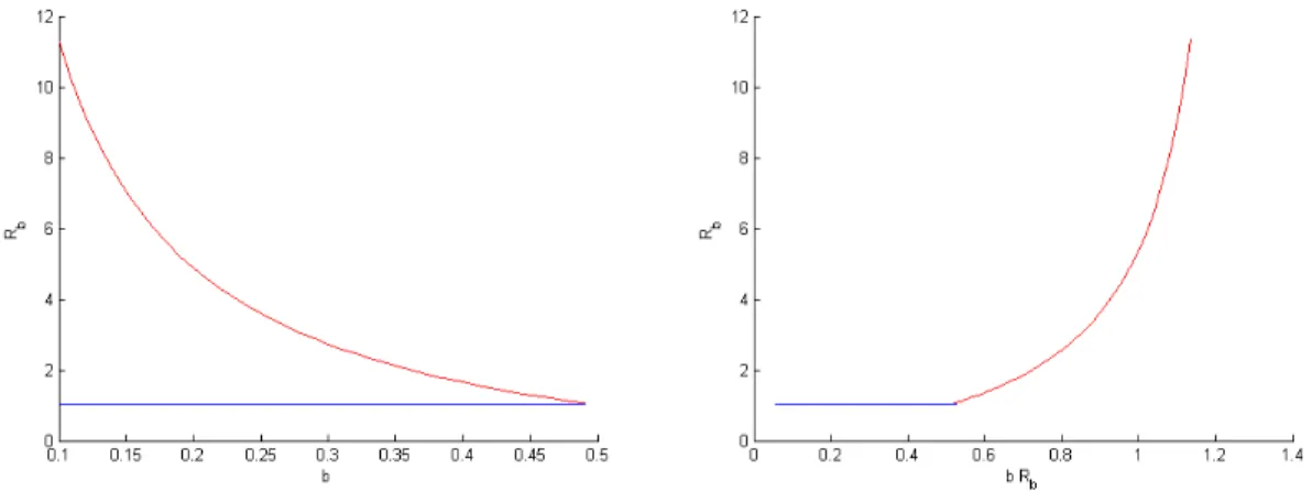
Figure 2: Interest Rate Schedules for b and bRb

In Figure 2, the two classes of schedules above are depicted. Calvo schedules are presented on the left panel, and Arellano schedules on the right panel. As can be seen, on the left panel, there is not a single schedule. In fact, there are two types of schedules, the “good” equilibrium schedule (blue) and the “bad” equilibrium schedule (red), and they cannot be oﬀered at the same time.8 _This

happens as a schedule is a function and in the left panel we do not have one, there are two interest rates for each level of debt. This is, in fact, where expectations play an important role. Depending on what investors expect (or know as I am considering perfect foresight), they will present one of those schedules. In this sense, if investors believe that there will be an haircut, the red schedule will be presented. If they believe there will be no haircut, the blue schedule will be presented.9

8_{They are called good and bad schedule for two reasons: first in the good schedule the level}

of taxes is lower and so welfare is higher, secondly there is no haircut in the good schedule.

(20)

In the right panel we have, again, both schedules depicted, but now for the case when investors coordinate upon promised repayment at maturity. In this case, as can easily be seen, in spite of having both schedules we have a single one as both of them combined are still represented by a function. There is a unique Rb for each level of bRb, which is debt at maturity.

4.3 Numerical Results and Equilibria

It is now possible to see whether multiplicity exists for both classes of sched-ules, and so for two diﬀerent definitions of equilibrium. For that, as I am still considering the assumption of a competitive government, we need to look at the intersection of demand with the interest rate schedules.

Equilibrium (Competitive) with Calvo schedules An equilibrium is (e✓, eb, eRb) such that: given eRb, (i) the government chooses the amount of debt, eb,

in period 0 in order to maximize utility subject to the resources constraints and arbitrage condition (4), as in (13); (ii) the government chooses the fraction of debt repudiated, e✓, in period 1 in order to maximize utility in period 1 subject to the resources constraint for that period, as in (12); (iii) both government budget constraints are satisfied with x⇤

0 and x⇤1being pinned down with the choice of eb and

e

✓ and; (iv) the arbitrage condition (5) is satisfied when investors oﬀer a schedule. To get the demand function for the case of debt at maturity one could think that instead of solving the problem in (13), one would define the problem in the variable of interest, bq _{= bR}

b also knowing that q = _R1_b:

maxbqU (c₀, c₁) s.t.

y0 = c0+ k1 k0R + g0+ z(g0 qbq)

y1 = c1 k1R + g1 + ↵✓bbq+ z(g1 + bq(1 ✓b) + ↵✓bbq)

R = 1

(16)

The result would be the same if one would simply replace bRb = bq in (15) as

this is simply a change of variables.

(21)

The same change of variables can be done to equation (5) so that: R = 1

q(1 ✓) (17)

Equilibrium (Competitive) with Arellano schedules An equilibrium is (e✓, ebq_, _q)_e _{such that: given eq, (i) the government chooses debt at maturity, eb}q_,

in period 0 in order to maximize utility subject to the resources constraints and arbitrage condition (4), as in (16); (ii) the government chooses the fraction of debt repudiated, e✓, in period 1 in order to maximize utility in period 1 subject to the resources constraint for that period, as in (12); (iii) both government budget constraints are satisfied with x⇤

0 and x⇤1 being pinned down with the choice of ebq

and e✓ and; (iv) the arbitrage condition (17) is satisfied when investors oﬀer a schedule.

4.3.1 Large Public Expenditure in Period 0

In order to get to a solution one needs to do a simulation. Table 1 presents the first scenario considered: large government spending in period 0.

Parameter Value Description

↵ 0.4 Per capita cost of repudiation

R 1.05 Interest factor on asset without possibility of default 1 Coeﬃcient of marginal distortion of taxes

g0 1.5 Public expenditure in period 0

x⇤

1 0.(6) Optimal level of taxes in period 1

Table 1: Large public expenditure in period 0

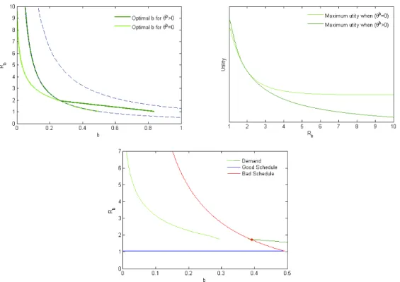
To get to the equilibrium interest rates and levels of debt, one needs to look at the intersection of the demand with the schedules. In the left panel of Figure 3, one can see the levels of debt that maximize utility, for each Rb, and either ✓ = 0

or ✓ > 0, as in (15). The government, knowing the interest rate and the way choosing b defines ✓, can choose which of the two debt levels maximizes utility. There should be just one level of debt that maximizes utility, given the interest rate and the feedback of that choice on the optimal haircut. In the right panel

(22)

of Figure 3, one can see the maximum utility attainable given that either there is no haircut or there is a positive haircut. From this, it can be seen that for high interest rates the maximum utility is attained with no haircut. However, for low interest rates, maximum utility is higher with a positive haircut. This happens as the haircut reduces government’s repayment towards investors which, in turns, leads to a higher optimal level of debt. The higher haircut, in this case, more than oﬀsets the higher repayment, in terms of utility. This is only true when interest rates are relatively low. Once the interest rates get higher, the higher repayment more than oﬀsets the positive haircut. This leads to the demand curve as in Figure 3.

Figure 3: Demand for debt and Equilibrium (Competitive) in Calvo’s class of schedules

Before going a step further, it is important to clarify that, as in Calvo (1988), these two schedules exist for x⇤

1 > g1+ bR. If x⇤1 = g1+ bRthen there would only

be one equilibrium (the good one) and if x⇤

1 < g1 + bR then there would be no

(23)

b = bmax = x⇤1 g1

R (18)

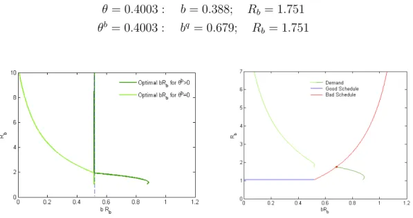
As can be seen in Figures 3 and 4, there is only the bad equilibrium: ✓ = 0.4003 : b = 0.388; Rb = 1.751

✓b _{= 0.4003 :} _bq _{= 0.679;} _R

b = 1.751

Figure 4: Demand for debt and Equilibrium (Competitive) in Arellano’s class of schedules

In this scenario the existence of a positive haircut, that reduces the repayment, more than oﬀsets the higher interest rate, in utility terms.

4.3.2 Small Public Expenditure in Period 0

Table 2 presents the second scenario considered: a small public expenditure in period 0.

Parameter Value Description

↵ 0.4 Per capita cost of repudiation

R 1.05 Interest factor on asset without possibility of default 1 Coeﬃcient of marginal distortion of taxes

x⇤

1 0.(6) Optimal level of taxes in period 1

(24)

I follow the same approach as in scenario 1. Changing the amount of public spending changes also the optimal choice of debt, for each interest rate. Again, there are two levels of debt for each Rb as in (15): one for a positive haircut and

the other for the case of no haircut. Looking at the utility for each level of debt and corresponding interest rate, for both cases, as in the top panel of Figure 5, it can be seen that the optimal level of debt for ✓ = 0 is always better than the other, in terms of utility. This leads to the demand curve, as in Figure 5.

Figure 5: Equilibrium (Competitive) with small public expenditure in period 0 In this case there is also a single equilibrium: the good equilibrium.

✓ = 0 : b = 0.2927; Rb = R = 1.05

Alternatively, one can also look at the equilibrium debt levels and interest rates for coordination upon debt at maturity:

(25)

Summing up, in this case there are no multiple equilibria. If the good schedule is oﬀered, there is one equilibrium interest rate and debt level. However, if the bad schedule is oﬀered there is no equilibrium. It seems that, as spending is low, there are not enough incentives for the government to bear a high interest rate in order to get indebted.

It is interesting to see the impact of ↵ on these results. In fact, a lower ↵ means that the cost of repudiating debt is lower. In this sense, g0 would not need

to be as high in order to obtain an equilibrium in the bad schedule. The reverse is true for a higher ↵. Having said so, a change of ↵ would only mean a diﬀerent starting point for public expenditure in order to obtain the same results.

5 The Case of a Government as a Large Agent

In this section, after seeing what would happen if the government behaved in a competitive way, I present the results for a government behaving as a large agent, meaning that now it does not take Rb as given, but Rb(b), the entire schedule.

This new setting can be described as a dynamic game in which the leader, the government, decides how much to borrow and investors reply with an interest rate. The government can anticipate investors’ decisions, thus being able to plug in their best response, Rb(b), in Rb while choosing b. A big agent takes into

account that his decisions impact the solution, in this case, the interest rate.

5.1 Problem Definition and Solution

To solve the problem I use the same method as in section 4, backwards induction. In this sense, the only important change is the fact that the government takes the interest rate schedule, Rb(b) as given instead of the interest rate itself. Now,

the government takes into account all equilibrium conditions when choosing the level of debt. The timing is the same as in section 4. Now there is no demand curve. Instead, the government chooses the point in the schedule (level of debt and corresponding interest rate) that maximizes utility.

The first step of the maximization problem in (9), which first-order condition is presented in (10), also applies here. This happens as in period 1, b and Rb

(26)

are already decided, and so the government is choosing ✓ knowing what happens before that period. Wether the government takes the interest rate or the interest rate schedule as given does not make any diﬀerence in terms of b and Rb, as they

are already decided. Having said so, there still is ✓b _{as in (14). The diﬀerence}

appears when the government decides the amount of debt in period 0. Now, instead of only replacing ✓ for ✓b_{, replacing R}

b for each type of schedule, for both

classes, is also needed. A big government takes into account all the equilibrium conditions while maximizing.

Bearing in mind that there is no demand curve, in the following subsections the focus of the analysis is on the diﬀerent classes and types of schedules.

5.1.1 Calvo Schedules

I begin the analysis for the class of schedules Rb(b), as implicitly defined in Calvo

(1988). As was already said, depending on investor’s expectations there are dif-ferent types of schedules presented. In this sense, for each of the schedules, the government chooses a debt level and interest rate, as it takes Rb(b) as given.

If the schedule presented is the blue one, then Rb(b) = R. Plugging in Rb(b)

as well as ✓ = 0 in (13) and taking derivatives with respect to b one gets to the optimal level of debt. Looking at (15) this is the same level of debt if we simply substitute Rb for R in the first branch of demand, the one in which ✓ = 0. In

Section 4, I did not replace ✓ = 0 as the condition Rb(1 ✓) = R, solved by the

schedule, was not taken into consideration by a competitive government. A large government, however, takes that into consideration as the schedule is given. Thus, here, the first-order condition defines a unique value of b as g0 is exogenous and ↵

and R are parameters. The equilibrium itself is the same as in the competitive case as for this schedule taking the price as given is the same as taking the schedule as given (i.e. the schedule is a unique Rb for diﬀerent values of b) and in equilibrium

the arbitrage condition is satisfied, no matter if the agent is large or small. If the schedule presented is the red one, then Rb(b) = _{(1 ↵)b}1 g_↵b1 1 ↵_↵ R.10

Here, however, there is no interior solution. As b increases, as can be seen in Figure 6 below, bRb decreases and also, by (4) ✓ decreases. In this sense, the

(27)

cost of repudiation (↵✓bRb) decreases for both reasons: there is less to repay

(i.e. less to default on), and the haircut is getting smaller. One could think that the decrease in ✓ could oﬀset the decrease of bRb, thus increasing x1, which

would decrease utility. However, the variations of ✓ just oﬀset the variations of debt repayment, such that x⇤

1 is constant. Having said this, increasing b in the

bad schedule decreases the cost of defaulting, does not change taxes in period 1, and decreases taxes in period 0, for the same amount of government spending. Summing up the eﬀects, increasing b is welfare improving in this schedule. Thus, the government, having the ability to choose the amount of debt, chooses the maximum amount of debt possible.

Figure 6: Level of debt versus debt at maturity

Having said this, an optimizing large government chooses debt so that the constraint b  x1 g1

R is active as in (18). Again, this is a unique value of b for the

same reason as above.

5.1.2 Arellano Schedules

The next logical step is to look at the class of schedules Rb(bq), where bq = bRb.

As said before, investors present a single schedule that comprises both the blue and the red schedule. The process is the same as in the previous subsection in the sense that the government will choose a pair (bq_{, R}

b) as it takes Rb(bq) as

given. The diﬀerence is that here the government is choosing the amount of debt it promises to pay at maturity.

(28)

Here there is no sense in distinguishing the types of schedules as both can be oﬀered as a single one. Having said so, the government will always choose the equilibrium in the good schedule as it yields a better outcome compared to the outcome of the bad equilibrium. In the good equilibrium Rb = R, but bR is lower

(or equal) than the minimum repayment in the bad schedule, bq _{= bR}

b. For the

good equilibrium, the reasoning is the same as in the subsection above. Knowing already the level of debt that the government would choose and the interest rate contracted, bq _{= bR} _{is also pinned down.}

5.2 Numerical Results and Equilibria

In this setting the government, given the schedule, is able to choose the amount of debt that maximizes utility. In the competitive case, the government had to contract a certain amount of debt, taking the interest rate as given, here the government can choose given the schedule.

Equilibrium with Calvo Schedules An equilibrium is a schedule eRb(b) and

(e✓, eb, eRb)such that: given the schedule, (i) the government chooses the amount of

debt, eb, in period 0 in order to maximize utility subject to the resources constraints and to the arbitrage condition (4); (ii) the government chooses the fraction of debt repudiated, e✓, in period 1 in order to maximize utility in period 1 subject to the resources constraint for that period, as in (12); (iii) both government budget constraints are satisfied with x⇤

0 and x⇤1 being pinned down with the choice of eb

and e✓; (iv) the schedule solves the arbitrage condition (5) and; (v) eRb(eb) = eRb.

Equilibrium with Arellano Schedules An equilibrium is a schedule eRb(bq =

bRb)and (e✓, ⇠

bq_,_R⇠

b)such that: given the schedule, (i) the government chooses debt

at maturity, ebq_{, in period 0 in order to maximize utility subject to the resources}

constraints and to the arbitrage condition (4); (ii) the government chooses the fraction of debt repudiated, e✓, in period 1 in order to maximize utility in period 1 subject to the resources constraint for that period, as in (11); (iii) both government budget constraints are satisfied with x⇤

0 and x⇤1 being pinned down with the choice

of eb and e✓ and; (iv) the schedule solves the arbitrage condition (17) and; (v) e

(29)

5.2.1 Large Public Expenditure in Period 0

In order to obtain a solution the scenario as in Table 1 - large public expenditure in period 0 - is used first.

Let us start the analysis with Calvo’s class of schedules. The government is choosing b to maximize utility given Rb(b). In this sense, as there are two types

of schedules, depending on investors’ beliefs on the existence of an haircut, there could be two equilibria. In the good equilibrium, there is no haircut, in the bad one, the government chooses the level of debt that provides the same interest rate as in the blue schedule, meaning that ✓ is also 0. In this particular scenario, both in the good and bad equilibrium there is a corner solution. In the good equilibrium because of the high expenditure, in the bad equilibrium because the government wants to minimize the promised debt repayment given that it got the bad schedule. In this sense, there is only one equilibrium regardless of the schedule presented.

Figure 7: Equilibria with high public expenditure in period 0

✓ = 0 : b = bmax = 0.492; Rb = R = 1.05

In Arellano’s class of schedules the same unique solution is found. In the next subsection I will focus on the argument of existence of a unique solution for Arellano schedules as in this class there is only one schedule, comprised by both the good and the bad schedule.

(30)

5.2.2 Small Public Expenditure in Period 0

In this subsection, I use, again, Table 2 - small government expenditure in period 0. Starting the analysis with Calvo’s class of schedules, it can be seen that for a small expenditure, as is the case in this scenario, the equilibrium in the good schedule is not a corner solution. As the government behaves as a large agent and chooses a level of debt, and interest rate for a given schedule, there will also exist an equilibrium in the bad schedule. This is a corner solution for the same reasons stated above. In this sense, there is a diﬀerent unique equilibrium for each type of schedule meaning that for Calvo’s class of schedules, under this scenario, there is multiplicity depending on investors’ beliefs:

Good Equilibrium : ✓ = 0; b = 0.2927; Rb = R = 1.05

Bad Equilibrium : ✓ = 0; b = 0.492; Rb = R = 1.05

Figure 8: Equilibria with small public expenditure in period 0

In Arellano’s class of schedules there is a slight diﬀerence. As was said before, the schedule is unique and both types, the good and the bad, can be oﬀered altogether. In this sense, if the government has the possibility of choosing between two promised repayments, for the same interest rate, and given that the good equilibrium is the one with the lower repayment, it will always choose the latter. Thus, with this class of schedules and allowing the government to behave as a large agent, the equilibrium is indeed unique, no matter the magnitude of the exogenous government expenditure.

(31)

✓ = 0 : bq = 0.3073; Rb = R = 1.05

The issue here is that the way investors coordinate is not explained. Either investors coordinate as in Calvo (1988), or as in Arellano (2008). When investors coordinate on diﬀerent classes of schedules there are diﬀerent equilibrium debt levels - for not extreme levels of g0 as in this scenario. The way investors coordinate

could be seen as random.

The fact that changing the way the schedule is presented, and so the variable the government is choosing can bring uniqueness, provided that the government behaves as a large agent, could be anticipated by Figure 6. If the government is choosing b there can be two possible bq_{. However, if the government is choosing b}q

there is only one b that provides that promised payment. This happens as, when choosing bq_{, knowing R}

b and ✓b(b, Rb), there is also one unique value of b.

6 Concluding Remarks

This article has considered in detail not only the role of expectations, but also the role of government’s behavior when choosing the amount of debt in period 0, and even the role of investors’ coordination on presenting a schedule, on multiplicity of equilibria.

In Calvo’s setting, I found that, if the government behaves as a competitive agent, there is a single equilibrium. This result does not depend on the class of schedules oﬀered by investors. However, depending on the dimension of exogenous spending there are diﬀerent equilibrium interest rates, debt levels and haircuts. When public expenditures are large, the government has incentives to borrow. As public spending decreases so do the incentives. In this sense, in the large public debt scenario I found a single bad equilibrium. The latter exists as the government is willing to bear a higher interest rate in order to decrease the distortion in period zero, as without debt there would be higher taxes in period 0 and so a higher distortion. Another reason that makes it possible for the government to bear the interest rate is the existence of a positive haircut that reduces the repayment. The latter, in turn, is responsible for the high interest rate in the first place. In

(32)

this case, the haircut is such that utility is higher when compared to the case of no haircut. When public expenditures are small, government’s incentives to borrow at high interest rates are gone. As the government is no longer able to bear a higher interest rate in order to hold debt, the bad equilibrium no longer exists. There is a unique equilibrium: the good equilibrium. Regarding the class of schedules upon which investors coordinate, as the government is not a large agent and cannot choose directly the amount of debt, these do not influence the existence of one or more equilibria.

If the government behaves as a large agent, then the results are different. In this setting, with small expenditures, there is multiplicity as the government still has to pick the level of debt that maximizes utility for both good and bad schedules. So, depending on the type of schedule offered there is the good or the bad equilibrium. However, I found that, depending on the class of schedules investors offer, uniqueness can be achieved regardless of the magnitude of public spending. This is why in the beginning I stressed the importance of endogenizing debt: Letting the government behave as a large agent, while choosing the level of debt, and knowing that investors can coordinate on a schedule depending on debt at maturity, as in Arellano, then there is a unique equilibrium. In fact, a decision maker wanting to ensure a unique good equilibrium could do it by accepting only contracts on Arellano terms. If the contract was as in Calvo multiplicity would still exist, for not extreme values of g0. However, one cannot simply force investors

to coordinate in one way or the other.

Multiplicity arises from the lack of commitment of the government and from the expectations that are built afterwards regarding the haircut. In other words, multiplicity arises from the multiple schedules that can be oﬀered by investors. With endogenous debt and the government behaving as a large agent, which is usually the case, there are mixed results. If, by chance, investors were to present the case that ensures uniqueness we would have it. However, it is a long shot.

(33)

7 Appendix

Appendix A

In order to define the problem in section 3.1, one needs to get the resources constraint. For that I plug in taxes from the government budget constraint into the household’s budget constraint as follows:

8 < : y1+ k1R + bRb(1 ✓) = c1+ x1+ z(x1) x1 = g1+ bRb(1 ✓) + ↵✓bRb , , y1 = c1 k1R + g1+ ↵✓bRb+ z(g1+ bRb(1 ✓) + ↵✓bRb)

Now, the problem is defined as follows: max✓U (c1)

s.t. y1 = c1 k1R + g1+ ↵✓bRb+ z(g1+ bRb(1 ✓) + ↵✓bRb)

Taking derivatives with respect to ✓, after plugging in the constraint, and taking into account that, in period 1, Rb is known (and b is exogenous), g1 and y1

are exogenous, we get, for the linear case:

(✓) ↵bRb+ z0(g1+ bRb(1 ✓) + ↵✓bRb)⇥ ( bRb + ↵bRb) = 0,

, z0_(g

1+ bRb(1 ✓) + ↵✓bRb)⇥ bRb(1 ↵) = ↵bRb ,

, z0_(g

1+ bRb(1 ✓) + ↵✓bRb) = _{1 ↵}↵

This first-order condition implicitly defines a unique x⇤

1. However, the problem

in section 3.1 has two restrictions: 0  ✓  1. Substituting ✓ = 0 and ✓ = 1 in the government budget constraint one gets the following restrictions as depicted in Figure 1: 8 < : x1 = g1+ bRb(1 ✓) + ↵✓bRb x1 = g1+ bRb(1 ✓) + ↵✓bRb , 8 < : ✓ = 0 : x1 = g1+ bRb ✓ = 1 : x1 = g1+ ↵bRb

To get the equilibrium interest rates, the arbitrage condition and the govern-ment budget constraint in period 1 must also hold. Plugging in one in the other one gets the consistency condition:

(34)

8 < : x1 = g1+ bRb(1 ✓) + ↵✓bRb Rb(1 ✓) = R , 8 < : x1 = g1+ bRb ⇣ Rb Rb+R Rb ⌘ + ↵Rb R Rb bRb ✓ = Rb R Rb , x1 = g1+ bR + ↵bRb ↵bR , , x1 = g1+ (1 ↵)bR + ↵bRb

Equilibrium interest rates are found as in Figure 1 when x1 = x⇤1 or ✓ = 0 and

the consistency condition is satisfied.

Appendix B

To solve the problem defined in section 4.1, as stated above, we will use backwards induction. First we need to solve

max✓U (c1)

s.t. y1 = c1 k1R + g1+ ↵✓bRb+ z(g1+ bRb(1 ✓) + ↵✓bRb)

Which yields the same first-order condition as in Appendix A: z0_(g

1+ bRb(1 ✓) + ↵✓bRb) = _{1 ↵}↵

Knowing x⇤

1, through the government budget constraint and the function z(x),

we also know ✓b_{, as a function of b and R}

b. In this sense, in period 0, the

govern-ment will decide how much debt it borrows, knowing that ✓ = ✓b_{. Then, we need}

to solve

maxb c0+ _R1c1

s.t. y0 = c0+ k1 k0R + g0+ z(g0 b)

y1 = c1 k1R + g1+ ↵✓bbRb+ z(g1+ bRb(1 ✓b) + ↵✓bbRb)

Taking derivatives with respect to b we get: (b) z0_(g 0 b) +_R1↵✓bRb+ _R1↵bRb@✓ b @b + 1 R⇥ z0(g1+ bRb(1 ✓ b_{) + ↵✓}b_bR b)⇥ ⇥(Rb Rb✓b bRb@✓ b @b + ↵✓ b_R b + ↵bRb@✓ b @b) = 0

For the sake of simplicity I use z(x) = ₂x2_, _{> 0, and thus, z}0_{(x) = x. In}

this sense, from the first order condition when taking derivatives with respect to ✓ we get x⇤1 = (1 ↵)↵ . More than that, we get:

(35)

z0_(x 1) = g1+ bRb(1 ✓) + ↵✓bRb = _{(1 ↵)}↵ , , ✓(↵bRb bRb) = _{(1 ↵)}↵ g1 bRb , , ✓b ₌⇣ ↵ (1 ↵) g1 bRb ⌘ 1 (↵ 1)bRb

This expression for ✓b _{is valid for 0 < ✓ < 1:}

✓ = 0_{) bR}b = _{(1 ↵)}↵ g1, if g1 < _{(1 ↵)}↵ ✓ = 1_{) bR}b = _{(1 ↵)}1 g_↵1, if g1 < _{(1 ↵)}↵ ↵ (1 ↵) g1 < bRb < 1 (1 ↵) g1 ↵, if g1 < ↵ (1 ↵)

Thus, ✓b _{is defined as follows,}

✓b ₌ 8 > > > < > > > : 0 ⇣ ↵ (1 ↵) g1 bRb ⌘ 1 (↵ 1)bRb 1 , , , bRb  _{(1 ↵)}↵ g1 ↵ (1 ↵) g1 < bRb < 1 (1 ↵) g1 ↵ bRb _{(1 ↵)}1 g_↵1

Knowing the specification of ✓b _{we can solve the second step of the}

maximiza-tion problem:

maxb z(g0 b) _R1↵✓bbRb _R1 ⇥ z(g1+ bRb(1 ✓b) + ↵✓bbRb)

To get the demand when ✓b _{= 0}_{, taking derivatives with respect to b,} @z

@b = @z @x @x @b, one gets: (b) (g0 b) _R1 ⇥ (g1+ bRb)⇥ Rb = 0, b(1 + R2 b R) = g0 Rb Rg1 , , b = g0 Rb_Rg1 1+R2b R = Rg0 Rbg1 R+R2 b For ✓b ₌⇣ ↵ (1 ↵) g1 bRb ⌘ 1 (↵ 1)bRb, we get: (b) (g0 b) +_R1 _{↵ 1}↵ Rb ⇥ _R1 ⇥hg1+ bRb _{↵ 1}1 ⇣ ↵ (1 ↵) g1 bRb ⌘ +_{↵ 1}↵ ⇣_{(1 ↵)}↵ g1 bRb ⌘i ⇥ ⇥(Rb +_{↵ 1}Rb _{↵ 1}↵ Rb) = 0

As Rb+_{↵ 1}Rb _{↵ 1}↵ Rb = _{↵ 1}1 [Rb ↵Rb+ (↵ 1)Rb] = 0 the first-order condition

(36)

(g0 b) + _{(↵ 1)R}↵ Rb = 0 ,

, Rb = g0(1 ↵_↵ )R R(1 ↵_↵ )b

Finally, for ✓b _{= 1, we would get:}

(b) (g0 b) _R1↵Rb _R1 (g1+ ↵bRb)⇥ ↵Rb = 0 , [R1 + (↵Rb) 2_{]b = g} 0 ↵Rb ↵Rbg1 , , b = g0 ↵Rb(1+g1) 1 R+(↵Rb)2

However, ✓b _{= 1} _{does not yield an equilibrium with a positive stock of bonds:}

✓b _{= 1}_{) R}

b = +1 ) b = 0

One needs to take into consideration the domain of each branch of ✓b _{in order}

to get the optimal level of debt for each Rb, and either ✓ = 0 or ✓ > 0. Thus,

taking derivatives is not enough to ensure that the maximum is attained. There can be corner solutions. When deriving in each branch and respective domain, taking into account the restrictions, then we get the following:

b = 8 > > > < > > > : Rg0 Rbg1 R+R2 b ↵ (1 ↵) Rb g1 Rb g0 _{(1 ↵) R}↵ Rb , , , A B C A : Rg0Rb _{(1 ↵)}↵ R2b < (1 ↵)↵ R g1R B : _{(1 ↵) R}↵ b g1 Rb > g0 ↵ (1 ↵) RRb _ ↵ (1 ↵) Rb g1 Rb < Rg0 Rbg1 R+R2 b C : ↵ (1 ↵) g1 < ⇣ g0 _{(1 ↵) R}↵ Rb ⌘ Rb < _{(1 ↵)}1 g_↵1

In Figure 3, one can see the optimal levels of debt depicted. There, it is possible to see the domains and also the corner solutions that are not seen by simply taking a derivative.

Appendix C

To solve the problem defined in section 5.1, as stated above, we will use backwards induction. The first step is identical to the one in Appendix B. This appendix is relevant when plugging in the schedule in Rb. For the good schedule of Calvo’s

(37)

class of schedules, Rb(b) = R (and so ✓ = 0), the solution is the first branch of

the demand with Rb = R:

b = Rg0 Rbg1 R+R2 b = R(g0 g1) R(1+R) = g0 g1 1+R

In order to get the bad schedule, one needs to look at the intersection of x⇤₁ = _{(1 ↵)}↵ with the consistency condition x1 = g1 + bR(1 ↵) + ↵bRb, as in

Figure 1. ↵ (1 ↵) = g1+ bR(1 ↵) + ↵bRb , Rb(b) = 1 (1 ↵) b g1 ↵b 1 ↵ ↵ R

For this schedule the analysis is diﬀerent. The problem we are looking at is the following:

maxb z(g0 b) ↵✓bbRb(b) z(g1+ bRb(b)(1 ✓b) + ↵✓bbRb(b))

From Figure 1 one can see that in the bad equilibrium x1 = x⇤1 which is

con-stant. In this sense, whatever value bRb(b) takes, ✓b is such that for an exogenous

level of expenditure x1 is indeed constant. This means that, when bRb varies the

distortion in period 1 is constant as ✓b _{cancels out those variations. In period 0,}

from (1) b = x0, as g0 is exogenous, and so b > 0 ) z(x0) < 0. In this

sense, an increase of b decreases the distortion in period 0.

The question now is what happens to the term concerning the cost of repudi-ation as until now increasing debt has benefits for the large benevolent agent.

Multiplying the schedule in order to get bRb(b) it follows:

bRb(b) = _{(1 ↵)}1 g_↵1 1 ↵_↵ Rb = ↵ (1 ↵)g_{↵(1 ↵)}1 1 ↵_↵ Rb

As ↵ 2 [0, 1[, it can be seen that the slope is negative meaning that higher debt leads to less repayment, which means that Rb is decreasing. Moreover, from

(4) Rb < 0) ✓ < 0 as R is constant. In this sense, we get that an increase in

debt lowers not only bRb but also ✓ meaning that the per capita cost of repudiation

decreases.

Having said this, there is a clear gain from increasing debt. Thus, there is no interior solution as a large government wants to use the maximum amount of debt possible when presented with the bad schedule.

(38)

References

[1] Arellano, Cristina, "Default Risk and Income Fluctuations in Emerging Economies", American Economic Review, June 2008, 98 (3), 690–712.

[2] Calvo, Guillermo A., "Servicing the Public Debt: the Role of Expectations", American Economic Review, September 1988, 78 (4), 647–61.

[3] Corsetti, Giancarlo and Dedola, Luca, “The Mystery of the Printing Press. Self-fulfilling Debt Crises and Monetary Sovereignty”, CEPR Discussion Paper DP9358, Center for Economic Policy Research, April 2013

[4] Eaton, Jonathan and Gersovitz, Mark, “Debt with Potential Repudiation: Theoretical and Empirical Analysis,” Review of Economic Studies, April 1981, 48 (2), 289–309.

[5] Lorenzoni, Guido and Werning, Ivan, “Slow Moving Debt Crisis”, mimeo, MIT. [6] Navarro, Gaston, Nicolini, Juan Pablo and Teles, Pedro, “Sovereign Default: