A HEAT TRANSFER
TEXTBOOK
THIRD
EDITION
John H. Lienhard IV / John H. Lienhard V
A HEAT TRANSFER
TEXTBOOK
THIRD
EDITION
Third Edition
by
John H. Lienhard IV
and
John H. Lienhard V
Phlogiston
Press
University of Houston 4800 Calhoun Road
Houston TX 77204-4792 U.S.A.
Professor John H. Lienhard V
Department of Mechanical Engineering Massachusetts Institute of Technology 77 Massachusetts Avenue
Cambridge MA 02139-4307 U.S.A.
Copyright ©2008 by John H. Lienhard IV and John H. Lienhard V All rights reserved
Please note that this material is copyrighted under U.S. Copyright Law. The authors grant you the right to download and print it for your personal use or for non-profit instructional use. Any other use, including copying,
distributing or modifying the work for commercial purposes, is subject to the restrictions of U.S. Copyright Law. International copyright is subject to the Berne International Copyright Convention.
The authors have used their best efforts to ensure the accuracy of the methods, equations, and data described in this book, but they do not guarantee them for any particular purpose. The authors and publisher offer no warranties or representations, nor do they accept any liabilities with respect to the use of this information. Please report any errata to the authors.
Lienhard, John H., 1930–
A heat transfer textbook / John H. Lienhard IV and John H. Lienhard V — 3rd ed. — Cambridge, MA : Phlogiston Press, c2008
Includes bibliographic references and index. 1. Heat—Transmission 2. Mass Transfer I. Lienhard, John H., V, 1961– II. Title TJ260.L445 2008
Published by Phlogiston Press Cambridge, Massachusetts, U.S.A.
This book was typeset in Lucida Bright and Lucida New Math fonts (designed by Bigelow & Holmes) using LATEX under the Y&Y TEX System.
For updates and information, visit:
http://web.mit.edu/lienhard/www/ahtt.html
This copy is:
This book is meant for students in their introductory heat transfer course — students who have learned calculus (through ordinary differential equa-tions) and basic thermodynamics. We include the needed background in fluid mechanics, although students will be better off if they have had an introductory course in fluids. An integrated introductory course in thermofluid engineering should also be a sufficient background for the material here.
Our major objectives in rewriting the 1987 edition have been to bring the material up to date and make it as clear as possible. We have substan-tially revised the coverage of thermal radiation, unsteady conduction, and mass transfer. We have replaced most of the old physical property data with the latest reference data. New correlations have been intro-duced for forced and natural convection and for convective boiling. The treatment of thermal resistance has been reorganized. Dozens of new problems have been added. And we have revised the treatment of turbu-lent heat transfer to include the use of the law of the wall. In a number of places we have rearranged material to make it flow better, and we have made many hundreds of small changes and corrections so that the text will be more comfortable and reliable. Lastly, we have eliminated Roger Eichhorn’s fine chapter on numerical analysis, since that topic is now most often covered in specialized courses on computation.
This book reflects certain viewpoints that instructors and students alike should understand. The first is that ideas once learned should not be forgotten. We have thus taken care to use material from the earlier parts of the book in the parts that follow them. Two exceptions to this are Chapter 10 on thermal radiation, which may safely be taught at any point following Chapter 2, and Chapter 11 on mass transfer, which draws only on material through Chapter 8.
We believe that students must develop confidence in their own ability to invent means for solving problems. The examples in the text therefore do not provide complete patterns for solving the end-of-chapter prob-lems. Students who study and absorb the text should have no unusual trouble in working the problems. The problems vary in the demand that they lay on the student, and we hope that each instructor will select those that best challenge their own students.
The first three chapters form a minicourse in heat transfer, which is applied in all subsequent chapters. Students who have had a previous integrated course thermofluids may be familiar with this material, but to most students it will be new. This minicourse includes the study of heat exchangers, which can be understood with only the concept of the overall heat transfer coefficient and the first law of thermodynamics.
We have consistently found that students new to the subject are greatly encouraged when they encounter a solid application of the material, such as heat exchangers, early in the course. The details of heat exchanger de-sign obviously require an understanding of more advanced concepts — fins, entry lengths, and so forth. Such issues are best introduced after the fundamental purposes of heat exchangers are understood, and we develop their application to heat exchangers in later chapters.
This book contains more material than most teachers can cover in three semester-hours or four quarter-hours of instruction. Typical one-semester coverage might include Chapters 1 through 8 (perhaps skipping some of the more specialized material in Chapters 5, 7, and 8), a bit of Chapter 9, and the first four sections of Chapter 10.
We are grateful to the Dell Computer Corporation’s STAR Program, the Keck Foundation, and the M.D. Anderson Foundation for their partial support of this project.
I The General Problem of Heat Exchange 1
1 Introduction 3
1.1 Heat transfer . . . 3
1.2 Relation of heat transfer to thermodynamics. . . 6
1.3 Modes of heat transfer . . . 10
1.4 A look ahead . . . 35
1.5 Problems . . . 36
Problems . . . 37
References . . . 46
2 Heat conduction concepts, thermal resistance, and the overall heat transfer coefficient 49 2.1 The heat diffusion equation . . . 49
2.2 Solutions of the heat diffusion equation. . . 58
2.3 Thermal resistance and the electrical analogy . . . 62
2.4 Overall heat transfer coefficient,U . . . 78
2.5 Summary . . . 86
Problems . . . 86
References . . . 96
3 Heat exchanger design 99 3.1 Function and configuration of heat exchangers . . . 99
3.2 Evaluation of the mean temperature difference in a heat exchanger. . . 103
3.3 Heat exchanger effectiveness . . . 120
3.4 Heat exchanger design. . . 126
Problems . . . 129
References . . . 136
II Analysis of Heat Conduction 139 4 Analysis of heat conduction and some steady one-dimensional
problems 141
4.1 The well-posed problem . . . 141
4.2 The general solution . . . 143
4.3 Dimensional analysis. . . 150
4.4 An illustration of dimensional analysis in a complex steady conduction problem . . . 159
4.5 Fin design. . . 163
Problems . . . 183
References . . . 190
5 Transient and multidimensional heat conduction 193 5.1 Introduction. . . 193
5.2 Lumped-capacity solutions . . . 194
5.3 Transient conduction in a one-dimensional slab . . . 203
5.4 Temperature-response charts . . . 208
5.5 One-term solutions . . . 218
5.6 Transient heat conduction to a semi-infinite region. . . 220
5.7 Steady multidimensional heat conduction . . . 235
5.8 Transient multidimensional heat conduction. . . 247
Problems . . . 252
References . . . 265
III Convective Heat Transfer 267 6 Laminar and turbulent boundary layers 269 6.1 Some introductory ideas . . . 269
6.2 Laminar incompressible boundary layer on a flat surface 276 6.3 The energy equation . . . 292
6.4 The Prandtl number and the boundary layer thicknesses 296 6.5 Heat transfer coefficient for laminar, incompressible flow over a flat surface . . . 300
6.6 The Reynolds analogy . . . 311
6.7 Turbulent boundary layers . . . 313
6.8 Heat transfer in turbulent boundary layers . . . 322
Problems . . . 330
7 Forced convection in a variety of configurations 341
7.1 Introduction. . . 341
7.2 Heat transfer to and from laminar flows in pipes . . . 342
7.3 Turbulent pipe flow . . . 355
7.4 Heat transfer surface viewed as a heat exchanger . . . 367
7.5 Heat transfer coefficients for noncircular ducts. . . 370
7.6 Heat transfer during cross flow over cylinders. . . 374
7.7 Other configurations . . . 384
Problems . . . 386
References . . . 393
8 Natural convection in single-phase fluids and during film condensation 397 8.1 Scope . . . 397
8.2 The nature of the problems of film condensation and of natural convection . . . 398
8.3 Laminar natural convection on a vertical isothermal surface . . . 401
8.4 Natural convection in other situations . . . 416
8.5 Film condensation . . . 428
Problems . . . 443
References . . . 452
9 Heat transfer in boiling and other phase-change configurations 457 9.1 Nukiyama’s experiment and the pool boiling curve . . . 457
9.2 Nucleate boiling. . . 464
9.3 Peak pool boiling heat flux . . . 472
9.4 Film boiling . . . 486
9.5 Minimum heat flux. . . 488
9.6 Transition boiling and system influences . . . 489
9.7 Forced convection boiling in tubes . . . 496
9.8 Forced convective condensation heat transfer . . . 505
9.9 Dropwise condensation. . . 506
9.10 The heat pipe . . . 509
Problems . . . 513
IV Thermal Radiation Heat Transfer 523
10 Radiative heat transfer 525
10.1 The problem of radiative exchange. . . 525
10.2 Kirchhoff’s law. . . 533
10.3 Radiant heat exchange between two finite black bodies . 536 10.4 Heat transfer among gray bodies . . . 549
10.5 Gaseous radiation . . . 563
10.6 Solar energy . . . 574
Problems . . . 584
References . . . 592
V Mass Transfer 595 11 An introduction to mass transfer 597 11.1 Introduction. . . 597
11.2 Mixture compositions and species fluxes . . . 600
11.3 Diffusion fluxes and Fick’s law . . . 608
11.4 Transport properties of mixtures . . . 614
11.5 The equation of species conservation. . . 627
11.6 Mass transfer at low rates . . . 635
11.7 Steady mass transfer with counterdiffusion. . . 648
11.8 Mass transfer coefficients at high rates of mass transfer. 654 11.9 Simultaneous heat and mass transfer. . . 663
Problems . . . 673
References . . . 686
VI Appendices 689 A Some thermophysical properties of selected materials 691 References . . . 694
B Units and conversion factors 721 References . . . 722
C Nomenclature 725
Citation Index 733
The General Problem of Heat
Exchange
The radiation of the sun in which the planet is incessantly plunged, pene-trates the air, the earth, and the waters; its elements are divided, change direction in every way, and, penetrating the mass of the globe, would raise its temperature more and more, if the heat acquired were not exactly balanced by that which escapes in rays from all points of the surface and expands through the sky. The Analytical Theory of Heat, J. Fourier
1.1
Heat transfer
People have always understood that something flows from hot objects to cold ones. We call that flowheat. In the eighteenth and early nineteenth centuries, scientists imagined that all bodies contained an invisible fluid which they called caloric. Caloric was assigned a variety of properties, some of which proved to be inconsistent with nature (e.g., it had weight and it could not be created nor destroyed). But its most important feature was that it flowed from hot bodies into cold ones. It was a very useful way to think about heat. Later we shall explain the flow of heat in terms more satisfactory to the modern ear; however, it will seldom be wrong to imagine caloric flowing from a hot body to a cold one.
The flow of heat is all-pervasive. It is active to some degree or another in everything. Heat flows constantly from your bloodstream to the air around you. The warmed air buoys off your body to warm the room you are in. If you leave the room, some small buoyancy-driven (orconvective) motion of the air will continue because the walls can never be perfectly isothermal. Such processes go on in all plant and animal life and in the air around us. They occur throughout the earth, which is hot at its core and cooled around its surface. The only conceivable domain free from heat flow would have to be isothermal and totally isolated from any other region. It would be “dead” in the fullest sense of the word — devoid of any process of any kind.
The overall driving force for these heat flow processes is the cooling (or leveling) of the thermal gradients within our universe. The heat flows that result from the cooling of the sun are the primary processes that we experience naturally. The conductive cooling of Earth’s center and the ra-diative cooling of the other stars are processes of secondary importance in our lives.
The life forms on our planet have necessarily evolved to match the magnitude of these energy flows. But while “natural man” is in balance with these heat flows, “technological man”1has used his mind, his back, and his will to harness and control energy flows that are far more intense than those we experience naturally. To emphasize this point we suggest that the reader make an experiment.
Experiment 1.1
Generate as much power as you can, in some way that permits you to measure your own work output. You might lift a weight, or run your own weight up a stairwell, against a stopwatch. Express the result in watts (W). Perhaps you might collect the results in your class. They should generally be less than 1 kW or even 1 horsepower (746 W). How much less might be surprising.
Thus, when we do so small a thing as turning on a 150 W light bulb, we are manipulating a quantity of energy substantially greater than a human being could produce in sustained effort. The power consumed by an oven, toaster, or hot water heater is an order of magnitude beyond our capacity. The power consumed by an automobile can easily be three orders of magnitude greater. If all the people in the United States worked continuously like galley slaves, they could barely equal the output of even a single city power plant.
Our voracious appetite for energy has steadily driven the intensity of actual heat transfer processes upward until they are far greater than those normally involved with life forms on earth. Until the middle of the thirteenth century, the energy we use was drawn indirectly from the sun
1Some anthropologists think that the termHomo technologicus(technological man)
using comparatively gentle processes — animal power, wind and water power, and the combustion of wood. Then population growth and defor-estation drove the English to using coal. By the end of the seventeenth century, England had almost completely converted to coal in place of wood. At the turn of the eighteenth century, the first commercial steam engines were developed, and that set the stage for enormously increased consumption of coal. Europe and America followed England in these developments.
The development of fossil energy sources has been a bit like Jules Verne’s description inAround the World in Eighty Days in which, to win a race, a crew burns the inside of a ship to power the steam engine. The combustion of nonrenewable fossil energy sources (and, more recently, the fission of uranium) has led to remarkably intense energy releases in power-generating equipment. The energy transferred as heat in a nuclear reactor is on the order ofone million watts per square meter.
A complex system of heat and work transfer processes is invariably needed to bring these concentrations of energy back down to human pro-portions. We must understand and control the processes that divide and diffuse intense heat flows down to the level on which we can interact with them. To see how this works, consider a specific situation. Suppose we live in a town where coal is processed into fuel-gas and coke. Such power supplies used to be common, and they may return if natural gas supplies ever dwindle. Let us list a few of the process heat transfer problems that must be solved before we can drink a glass of iced tea.
• A variety of high-intensity heat transfer processes are involved with combustion and chemical reaction in the gasifier unit itself.
• The gas goes through various cleanup and pipe-delivery processes to get to our stoves. The heat transfer processes involved in these stages are generally less intense.
• The gas is burned in the stove. Heat is transferred from the flame to the bottom of the teakettle. While this process is small, it is intense because boiling is a very efficient way to remove heat.
• The steam passes through a turbine where it is involved with many heat transfer processes, including some condensation in the last stages. The spent steam is then condensed in any of a variety of heat transfer devices.
• Cooling must be provided in each stage of the electrical supply sys-tem: the winding and bearings of the generator, the transformers, the switches, the power lines, and the wiring in our houses.
• The ice cubes for our tea are made in an electrical refrigerator. It involves three major heat exchange processes and several lesser ones. The major ones are the condensation of refrigerant at room temperature to reject heat, the absorption of heat from within the refrigerator by evaporating the refrigerant, and the balancing heat leakage from the room to the inside.
• Let’s drink our iced tea quickly because heat transfer from the room to the water and from the water to the ice will first dilute, and then warm, our tea if we linger.
A society based on power technology teems with heat transfer prob-lems. Our aim is to learn the principles of heat transfer so we can solve these problems and design the equipment needed to transfer thermal energy from one substance to another. In a broad sense, all these prob-lems resolve themselves into collecting and focusing large quantities of energy for the use of people, and then distributing and interfacing this energy with people in such a way that they can use it on their own puny level.
We begin our study by recollecting how heat transfer was treated in the study of thermodynamics and by seeing why thermodynamics is not adequate to the task of solving heat transfer problems.
1.2
Relation of heat transfer to thermodynamics
The First Law with work equal to zero
Figure 1.1 The First Law of Thermodynamics for a closed system.
rate basis:
Q
positive toward the system
= Wk
positive away from the system
+ dUdt
positive when the system’s energy increases
(1.1)
whereQ is the heat transfer rate andWk is the work transfer rate. They may be expressed in joules per second (J/s) or watts (W). The derivative
dU/dt is the rate of change of internal thermal energy, U, with time, t. This interaction is sketched schematically in Fig.1.1a.
The analysis of heat transfer processes can generally be done with-out reference to any work processes, although heat transfer might sub-sequently be combined with work in the analysis of real systems. Ifp dV
work is the only work occuring, then eqn. (1.1) is
Q=pdV dt +
dU
dt (1.2a)
This equation has two well-known special cases:
Constant volume process: Q= dU
dt =mcv dT
dt (1.2b)
Constant pressure process: Q= dH
dt =mcp dT
dt (1.2c)
where H ≡ U+pV is the enthalpy, andcv andcp are the specific heat
capacities at constant volume and constant pressure, respectively. When the substance undergoing the process is incompressible (so that
cv =cp ≡c. The proper form of eqn. (1.2a) is then
Q= dU dt =mc
dT
dt (1.3)
Since solids and liquids can frequently be approximated as being incom-pressible, we shall often make use of eqn. (1.3).
If the heat transfer were reversible, then eqn. (1.2a) would become2
T dS dt
Qrev
=pdV
dt
Wkrev
+dUdt (1.4)
That might seem to suggest thatQcan be evaluated independently for in-clusion in either eqn. (1.1) or (1.3). However, it cannot be evaluated using
T dS, because real heat transfer processes are all irreversible andSis not defined as a function ofTin an irreversible process. The reader will recall that engineering thermodynamics might better be named thermostatics, because it only describes the equilibrium states on either side of irre-versible processes.
Since the rate of heat transfer cannot be predicted using T dS, how can it be determined? IfU(t)were known, then (whenWk= 0) eqn. (1.3) would giveQ, butU(t)is seldom knowna priori.
The answer is that a new set of physical principles must be introduced to predictQ. The principles aretransport laws, which are not a part of the subject of thermodynamics. They include Fourier’s law, Newton’s law of cooling, and the Stefan-Boltzmann law. We introduce these laws later in the chapter. The important thing to remember is that a description of heat transfer requires that additional principles be combined with the First Law of Thermodynamics.
Reversible heat transfer as the temperature gradient vanishes
Consider a wall connecting two thermal reservoirs as shown in Fig.1.2. As long asT1> T2, heat will flowspontaneously andirreversibly from 1
to 2. In accordance with our understanding of the Second Law of Ther-modynamics, we expect the entropy of the universe to increase as a con-sequence of this process. IfT2 →T1, the process will approach being
quasistatic and reversible. But the rate of heat transfer will also approach 2T= absolute temperature,S= entropy,V= volume,p= pressure, and “rev” denotes
Figure 1.2 Irreversible heat flow between two thermal reservoirs through an intervening wall.
zero if there is no temperature difference to drive it. Thus all real heat transfer processes generate entropy.
Now we come to a dilemma: If the irreversible process occurs at steady state, the properties of the wall do not vary with time. We know that the entropy of the wall depends on its state and must therefore be constant. How, then, does the entropy of the universe increase? We turn to this question next.
Entropy production
The entropy increase of the universe as the result of a process is the sum of the entropy changes ofall elements that are involved in that process. The rate of entropy production of the universe, ˙SUn, resulting from the
preceding heat transfer process through a wall is ˙
SUn=S˙res 1+ S˙wall
=0, sinceSwall must be constant
+S˙res 2 (1.5)
where the dots denote time derivatives (i.e., ˙x≡dx/dt). Since the reser-voir temperatures are constant,
˙
Sres= Q
Tres. (1.6)
Now Qres 1 is negative and equal in magnitude to Qres 2, so eqn. (1.5)
becomes
˙
SUn=
Qres 1
1
T2 −
1
T1
The term in parentheses is positive, so ˙SUn >0. This agrees with
Clau-sius’s statement of the Second Law of Thermodynamics.
Notice an odd fact here: The rate of heat transfer,Q, and hence ˙SUn,
is determined by the wall’s resistance to heat flow. Although the wall is the agent that causes the entropy of the universe to increase, its own entropy does not change. Only the entropies of the reservoirs change.
1.3
Modes of heat transfer
Figure1.3shows an analogy that might be useful in fixing the concepts of heat conduction, convection, and radiation as we proceed to look at each in some detail.
Heat conduction
Fourier’s law. Joseph Fourier (see Fig. 1.4) published his remarkable bookThéorie Analytique de la Chaleurin 1822. In it he formulated a very complete exposition of the theory of heat conduction.
Hebegan his treatise by stating the empirical law that bears his name:
the heat flux,3q(W/m2),resulting from thermal conduction is proportional
to the magnitude of the temperature gradient and opposite to it in sign. If we call the constant of proportionality,k, then
q= −kdT
dx (1.8)
The constant,k, is called thethermal conductivity. It obviously must have the dimensions W/m·K, or J/m·s·K, or Btu/h·ft·◦F if eqn. (1.8) is to be dimensionally correct.
The heat flux is a vector quantity. Equation (1.8) tells us that if temper-ature decreases withx,qwill be positive—it will flow in thex-direction. If T increases with x, q will be negative—it will flow opposite the x -direction. In either case,qwill flow from higher temperatures to lower temperatures. Equation (1.8) is the one-dimensional form of Fourier’s law. We develop its three-dimensional form in Chapter 2, namely:
q= −k∇T
3The heat flux,q, is a heat rate per unit area and can be expressed asQ/A, whereA
ment official in Napoleonic France and he was also an applied mathe-matician of great importance. He was with Napoleon in Egypt between 1798 and 1801, and he was subsequently prefect of the administra-tive area (or “Department”) of Isère in France until Napoleon’s first fall in 1814. During the latter period he worked on the theory of heat flow and in 1807 submitted a 234-page monograph on the sub-ject. It was given to such luminaries as Lagrange and Laplace for review. They found fault with his adaptation of a series expansion suggested by Daniel Bernoulli in the eighteenth century. Fourier’s theory of heat flow, his governing differential equation, and the now-famous “Fourier series” solution of that equation did not emerge in print from the ensuing controversy until 1822. (Etching from Por-traits et Histoire des Hommes Utiles, Collection de Cinquante PorPor-traits, Société Montyon et Franklin 1839-1840).
Example 1.1
The front of a slab of lead (k=35 W/m·K) is kept at 110◦C and the back is kept at 50◦C. If the area of the slab is 0.4 m2 and it is 0.03 m
thick, compute the heat flux,q, and the heat transfer rate,Q.
Solution. For the moment, we presume thatdT /dx is a constant equal to(Tback−Tfront)/(xback −xfront); we verify this in Chapter 2.
Thus, eqn. (1.8) becomes
q= −35
50−110
0.03
= +70,000 W/m2=70 kW/m2
and
Q=qA=70(0.4)=28 kW
In one-dimensional heat conduction problems, there is never any real problem in deciding which way the heat should flow. It is therefore some-times convenient to write Fourier’s law in simple scalar form:
q=k∆T
L (1.9)
where Lis the thickness in the direction of heat flow and qand∆T are both written as positive quantities. When we use eqn. (1.9), we must remember thatqalways flows from high to low temperatures.
Figure 1.5 Heat conduction through gas separating two solid walls.
processes are more efficient in solids than they are in gases. Notice that
−dTdx = qk ∝ 1k
since, in steady conduction,qis
constant
(1.10)
Thus solids, with generally higher thermal conductivities than gases, yield smaller temperature gradients for a given heat flux. In a gas, by the way, k is proportional to molecular speed and molar specific heat, and inversely proportional to the cross-sectional area of molecules.
This book deals almost exclusively with S.I. units, orSystème Interna-tional d’Unités. Since much reference material will continue to be avail-able in English units, we should have at hand a conversion factor for thermal conductivity:
1= J
0.0009478 Btu· h 3600 s ·
ft 0.3048 m·
1.8◦F K
Thus the conversion factor from W/m·K to its English equivalent, Btu/h·
ft·◦F, is
1=1.731 W/m·K
Btu/h·ft·◦F (1.11)
Consider, for example, copper—the common substance with the highest conductivity at ordinary temperature:
kCu at room temp=(383 W/m·K)
1.731 W/m·K
The range of thermal conductivities is enormous. As we see from Fig.1.6,kvaries by a factor of about 105 between gases anddiamondat room temperature. This variation can be increased to about 107if we
in-clude the effective conductivity of various cryogenic “superinsulations.” (These involve powders, fibers, or multilayered materials that have been evacuated of all air.) The reader should study and remember the order of magnitude of the thermal conductivities of different types of materi-als. This will be a help in avoiding mistakes in future computations, and it will be a help in making assumptions during problem solving. Actual numerical values of the thermal conductivity are given in Appendix A (which is a broad listing of many of the physical properties you might need in this course) and in Figs.2.2and2.3.
Example 1.2
A copper slab (k= 372 W/m·K) is 3 mm thick. It is protected from corrosion on each side by a 2-mm-thick layer of stainless steel (k=17 W/m·K). The temperature is 400◦C on one side of this composite wall and 100◦C on the other. Find the temperature distribution in the copper slab and the heat conducted through the wall (see Fig.1.7).
Solution. If we recall Fig.1.5and eqn. (1.10), it should be clear that
the temperature drop will take place almost entirely in the stainless steel, where kis less than 1/20 of k in the copper. Thus, the cop-per will be virtually isothermal at the average temcop-perature of(400+ 100)/2=250◦C. Furthermore, the heat conduction can be estimated in a 4 mm slab of stainless steel as though the copper were not even there. With the help of Fourier’s law in the form of eqn. (1.8), we get
q= −kdT
dx ≃17 W/m·K·
400−100
0.004
K/m=1275 kW/m2
The accuracy of this rough calculation can be improved by con-sidering the copper. To do this we first solve for∆Ts.s.and∆TCu (see
Fig. 1.7). Conservation of energy requires that the steady heat flux through all three slabs must be the same. Therefore,
q=
k∆T L
s.s.=
k∆T L
Figure 1.7 Temperature drop through a copper wall protected by stainless steel (Example1.2).
but
(400−100)◦C ≡ ∆TCu+2∆Ts.s.
= ∆TCu 1+2(k/L)Cu (k/L)s.s.
= (30.18)∆TCu
Solving this, we obtain∆TCu = 9.94 K. So∆Ts.s. =(300−9.94)/2 =
145 K. It follows thatTCu, left=255◦C andTCu, right=245◦C.
The heat flux can be obtained by applying Fourier’s law to any of the three layers. We consider either stainless steel layer and get
q=17 W m·K
145 K
0.002 m =1233 kW/m
2
Thus our initial approximation was accurate within a few percent.
One-dimensional heat diffusion equation. In Example 1.2 we had to deal with a major problem that arises in heat conduction problems. The problem is that Fourier’s law involves two dependent variables, T and
q. To eliminate qand first solve for T, we introduced the First Law of Thermodynamics implicitly: Conservation of energy required thatqwas the same in each metallic slab.
Figure 1.8 One-dimensional heat conduction through a differ-ential element.
From Fourier’s law applied at each side of the element, as shown, the net heat conduction out of the element during general unsteady heat flow is
qnetA=Qnet= −kA∂ 2T
∂x2δx (1.12)
To eliminate the heat loss Qnet in favor of T, we use the general First
Law statement for closed, nonworking systems, eqn. (1.3):
−Qnet= dU
dt =ρcA
d(T−Tref)
dt δx=ρcA
dT
dtδx (1.13)
where ρ is the density of the slab and c is its specific heat capacity.4
Equations (1.12) and (1.13) can be combined to give
∂2T ∂x2 =
ρc k
∂T ∂t ≡
1
α ∂T
∂t (1.14)
4The reader might wonder ifcshould bec
porcv. This is a strictly incompressible
equation socp = cv =c. The compressible equation involves additional terms, and
Figure 1.9 The convective cooling of a heated body.
This is theone-dimensional heat diffusion equation. Its importance is this: By combining the First Law with Fourier’s law, we have eliminated the unknown Qand obtained a differential equation that can be solved for the temperature distribution,T (x, t). It is the primary equation upon which all of heat conduction theory is based.
The heat diffusion equation includes a new property which is as im-portant to transient heat conduction askis to steady-state conduction. This is the thermal diffusivity,α:
α≡ k ρc
J m·s·K
m3
kg kg·K
J =α m
2/s (or ft2/hr).
The thermal diffusivity is a measure of how quickly a material can carry heat away from a hot source. Since material does not just transmit heat but must be warmed by it as well, α involves both the conductivity, k, and the volumetric heat capacity,ρc.
Heat Convection
The physical process. Consider a typical convective cooling situation. Cool gas flows past a warm body, as shown in Fig. 1.9. The fluid imme-diately adjacent to the body forms a thin slowed-down region called a
boundary layer. Heat is conducted into this layer, which sweeps it away and, farther downstream, mixes it into the stream. We call such processes of carrying heat away by a moving fluidconvection.
In 1701, Isaac Newton considered the convective process and sug-gested that the cooling would be such that
dTbody
dt ∝Tbody−T∞ (1.15)
is constantly replenished, the body temperature need not change. Then with the help of eqn. (1.3) we get, from eqn. (1.15) (see Problem1.2),
Q∝Tbody−T∞ (1.16)
This equation can be rephrased in terms ofq=Q/Aas
q=hTbody−T∞
(1.17)
This is the steady-state form of Newton’s law of cooling, as it is usually quoted, although Newton never wrote such an expression.
The constanthis thefilm coefficientorheat transfer coefficient. The bar overh indicates that it is an average over the surface of the body. Without the bar, h denotes the “local” value of the heat transfer coef-ficient at a point on the surface. The units of h and h are W/m2K or
J/s·m2·K. The conversion factor for English units is:
1= 0.0009478 BtuJ ·1K
.8◦F·
3600 s
h ·
(0.3048 m)2
ft2 or
1=0.1761Btu/h·ft2·◦F
W/m2K (1.18)
It turns out that Newton oversimplified the process of convection when he made his conjecture. Heat convection is complicated and h
can depend on the temperature difference Tbody−T∞ ≡ ∆T. In Chap-ter6 we find thath really is independent of ∆T in situations in which fluid is forced past a body and∆T is not too large. This is calledforced convection.
When fluid buoys up from a hot body or down from a cold one, h
varies as some weak power of∆T—typically as ∆T1/4 or ∆T1/3. This is
calledfreeornatural convection. If the body is hot enough to boil a liquid surrounding it,hwill typically vary as∆T2.
For the moment, we restrict consideration to situations in which New-ton’s law is either true or at least a reasonable approximation to real behavior.
Table 1.1 Some illustrative values of convective heat transfer coefficients
Situation h, W/m2K
Natural convection in gases
• 0.3 m vertical wall in air,∆T =30◦C 4.33
Natural convection in liquids
• 40 mm O.D. horizontal pipe in water,∆T =30◦C 570
• 0.25 mm diameter wire in methanol,∆T =50◦C 4,000
Forced convection of gases
• Air at 30 m/s over a 1 m flat plate,∆T =70◦C 80
Forced convection of liquids
• Water at 2 m/s over a 60 mm plate,∆T =15◦C 590
• Aniline-alcohol mixture at 3 m/s in a 25 mm I.D. tube,∆T =80◦C 2,600
• Liquid sodium at 5 m/s in a 13 mm I.D. tube at 370◦C 75,000
Boiling water
• During film boiling at 1 atm 300
• In a tea kettle 4,000
• At a peak pool-boiling heat flux, 1 atm 40,000
• At a peak flow-boiling heat flux, 1 atm 100,000
• At approximate maximum convective-boiling heat flux, under
optimal conditions 106
Condensation
• In a typical horizontal cold-water-tube steam condenser 15,000
• Same, but condensing benzene 1,700
• Dropwise condensation of water at 1 atm 160,000
Example 1.3
The heat flux,q, is 6000 W/m2 at the surface of an electrical heater.
The heater temperature is 120◦C when it is cooled by air at 70◦C. What is the average convective heat transfer coefficient,h? What will the heater temperature be if the power is reduced so that qis 2000 W/m2?
Solution.
h= q
∆T =
6000
120−70 =120 W/m
2K
If the heat flux is reduced,hshould remain unchanged during forced convection. Thus
∆T =Theater−70◦C= q h =
2000 W/m2
120 W/m2K =16.67 K
soTheater=70+16.67=86.67◦C
Lumped-capacity solution. We now wish to deal with a very simple but extremely important, kind of convective heat transfer problem. The prob-lem is that of predicting the transient cooling of a convectively cooled object, such as we showed in Fig. 1.9. With reference to Fig. 1.10, we apply our now-familiar First law statement, eqn. (1.3), to such a body:
Q
−hA(T−T∞)
= dUdt
d
dt[ρcV (T−Tref)]
(1.19)
where A and V are the surface area and volume of the body, T is the temperature of the body,T =T (t), andTrefis the arbitrary temperature at whichUis defined equal to zero. Thus5
d(T −T∞)
dt = −
hA
ρcV(T−T∞) (1.20)
5Is it clear why(T−Tref)has been changed to(T−T
∞)under the derivative?
Remem-ber that the derivative of a constant (likeTreforT∞) is zero. We can therefore introduce
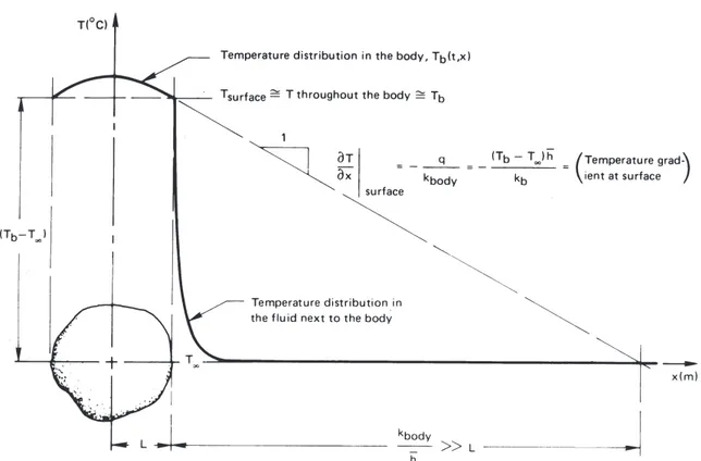
Figure 1.10 The cooling of a body for which the Biot number, hL/kb, is small.
The general solution to this equation is
ln(T−T∞)= − t
(ρcVhA) +C (1.21)
The groupρcVhAis thetime constant,T. If the initial temperature is
T (t=0)≡Ti, thenC=ln(Ti−T∞), and the cooling of the body is given
by
T−T∞ Ti−T∞ =
e−t/T (1.22)
The ratiot/T can also be interpreted as
t T =
hAt(J/◦C) ρcV (J/◦C) =
capacity for convection from surface
heat capacity of the body (1.23)
Notice that the thermal conductivity is missing from eqns. (1.22) and (1.23). The reason is that we have assumed that the temperature of the body is nearly uniform, and this means that internal conduction is not important. We see in Fig.1.10that, ifL(kb/ h)≪1, the temperature of
the body,Tb, is almost constant within the body at any time. Thus
hL kb ≪
1 implies that Tb(x, t)≃T (t)≃Tsurface
and the thermal conductivity,kb, becomes irrelevant to the cooling
pro-cess. This condition must be satisfied or the lumped-capacity solution will not be accurate.
We call the group hLkb the Biot number6, Bi. If Bi were large, of
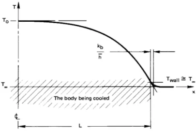
course, the situation would be reversed, as shown in Fig. 1.11. In this case Bi= hL/kb ≫ 1 and the convection process offers little resistance
to heat transfer. We could solve the heat diffusion equation
∂2T ∂x2 =
1
α ∂T
∂t
subject to the simple boundary conditionT (x, t) = T∞ whenx = L, to determine the temperature in the body and its rate of cooling in this case. The Biot number will therefore be the basis for determining what sort of problem we have to solve.
To calculate the rate of entropy production in a lumped-capacity sys-tem, we note that the entropy change of the universe is the sum of the entropy decrease of the body and the more rapid entropy increase of the surroundings. The source of irreversibility is heat flow through the boundary layer. Accordingly, we write the time rate of change of entropy of the universe,dSUn/dt≡S˙Un, as
˙
SUn=S˙b+S˙surroundings= −Qrev Tb +
Qrev T∞
6PronouncedBee-oh. J.B. Biot, although younger than Fourier, worked on the
Figure 1.11 The cooling of a body for which the Biot number, hL/kb, is large.
or
˙
SUn= −ρcV dTb dt
1
T∞−
1
Tb
.
We can multiply both sides of this equation bydtand integrate the right-hand side fromTb(t=0)≡Tb0toTbat the time of interest:
∆S= −ρcV
Tb
Tb0
1
T∞−
1
Tb
dTb. (1.24)
Equation1.24will give a positive∆SwhetherTb> T∞orTb< T∞because the sign ofdTb will always opposed the sign of the integrand.
Example 1.4
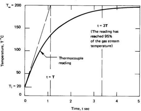
A thermocouple bead is largely solder, 1 mm in diameter. It is initially at room temperature and is suddenly placed in a 200◦C gas flow. The heat transfer coefficient h is 250 W/m2K, and the effective values
of k, ρ, and c are 45 W/m·K, 9300 kg/m3, and c = 0.18 kJ/kg·K,
Solution. The time constant,T, is
T = ρcV
hA =
ρc h
πD3/6
πD2 = ρcD
6h
= (9300)(60(250.18)()0.001) mkg3 kgkJ
·Km
m2·K
W
1000 W kJ/s
= 1.116 s
Therefore, eqn. (1.22) becomes
T−200◦C (20−200)◦C =e−
t/1.116 or T =200−180e−t/1.116◦C
This result is plotted in Fig.1.12, where we see that, for all practical purposes, this thermocouple catches up with the gas stream in less than 5 s. Indeed, it should be apparent that any such system will come within 95% of the signal in three time constants. Notice, too, that if the response could continue at its initial rate, the thermocouple would reach the signal temperature in one time constant.
This calculation is based entirely on the assumption that Bi ≪1 for the thermocouple. We must check that assumption:
Bi≡ hL
k =
(250 W/m2K)(0.001 m)/2
45 W/m·K =0.00278
This is very small indeed, so the assumption is valid.
Experiment 1.2
Invent and carry out a simple procedure for evaluating the time con-stant of a fever thermometer in your mouth.
Radiation
Figure 1.12 Thermocouple response to a hot gas flow.
Objects that are cooler than the fire, the toaster, or the sun emit much less energy because the energy emission varies as the fourth power of ab-solute temperature. Very often, the emission of energy, or radiant heat transfer, from cooler bodies can be neglected in comparison with con-vection and conduction. But heat transfer processes that occur at high temperature, or with conduction or convection suppressed by evacuated insulations, usually involve a significant fraction of radiation.
Experiment 1.3
Table 1.2 Forms of the electromagnetic wave spectrum
Characterization Wavelength,λ Cosmic rays < 0.3 pm Gamma rays 0.3–100 pm X rays 0.01–30 nm Ultraviolet light 3–400 nm Visible light 0.4–0.7 µm Near infrared radiation 0.7–30 µm Far infrared radiation 30–1000 µm
⎫ ⎪ ⎪ ⎪ ⎪ ⎬
⎪ ⎪ ⎪ ⎪ ⎭
Thermal Radiation 0.1–1000 µm
Millimeter waves 1–10 mm Microwaves 10–300 mm Shortwave radio & TV 300 mm–100 m Longwave radio 100 m–30 km
The electromagnetic spectrum. Thermal radiation occurs in a range of the electromagnetic spectrum of energy emission. Accordingly, it ex-hibits the same wavelike properties as light or radio waves. Each quan-tum of radiant energy has a wavelength,λ, and a frequency,ν, associated with it.
The full electromagnetic spectrum includes an enormous range of energy-bearing waves, of which heat is only a small part. Table1.2lists the various forms over a range of wavelengths that spans 17 orders of magnitude. Only the tiniest “window” exists in this spectrum through which we canseethe world around us. Heat radiation, whose main com-ponent is usually the spectrum of infrared radiation, passes through the much larger window—about three orders of magnitude inλorν.
Black bodies. The model for the perfect thermal radiator is a so-called
black body. This is a body which absorbs all energy that reaches it and reflects nothing. The term can be a little confusing, since such bodies
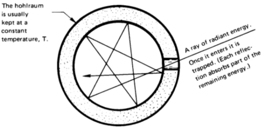
Figure 1.13 Cross section of a spherical hohlraum. The hole has the attributes of a nearly perfect thermal black body.
It is necessary to have an experimental method for making a perfectly black body. The conventional device for approaching this ideal is called by the German term hohlraum, which literally means “hollow space”. Figure1.13shows how a hohlraum is arranged. It is simply a device that traps all the energy that reaches the aperture.
What are the important features of a thermally black body? First consider a distinction between heat and infrared radiation. Infrared ra-diation refers to a particular range of wavelengths, whileheat refers to the whole range of radiant energy flowing from one body to another. Suppose that a radiant heat flux, q, falls upon a translucent plate that is not black, as shown in Fig. 1.14. A fraction, α, of the total incident energy, called the absorptance, is absorbed in the body; a fraction, ρ,
called thereflectance, is reflected from it; and a fraction, τ, called the
transmittance, passes through. Thus
1=α+ρ+τ (1.25)
This relation can also be written for the energy carried by each wave-length in the distribution of wavewave-lengths that makes up heat from a source at any temperature:
1=αλ+ρλ+τλ (1.26)
All radiant energy incident on a black body is absorbed, so that αb or
αλb = 1 and ρb = τb = 0. Furthermore, the energy emitted from a
black body reaches a theoretical maximum, which is given by the Stefan-Boltzmann law. We look at this next.
The Stefan-Boltzmann law. The flux of energy radiating from a body is commonly designatede(T )W/m2. The symbole
λ(λ, T) designates the
distribution function of radiative flux inλ, or themonochromatic emissive power:
eλ(λ, T )=
de(λ, T )
dλ or e(λ, T )=
λ
0 eλ(λ, T ) dλ (1.27)
Thus
e(T )≡E(∞, T )=
∞
0 eλ(λ, T ) dλ
The dependence of e(T ) onT for a black body was established experi-mentally by Stefan in 1879 and explained by Boltzmann on the basis of thermodynamics arguments in 1884. The Stefan-Boltzmann law is
eb(T )=σ T4 (1.28)
where the Stefan-Boltzmann constant,σ, is 5.670400×10⁻⁸ W/m2·K4
or 1.714×10⁻⁹Btu/hr·ft2·◦R4, andT is the absolute temperature.
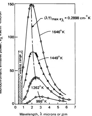
Figure 1.15 Monochromatic emissive power of a black body at several temperatures—predicted and observed.
white-hot, the energy distribution has been both greatly increased and shifted toward the shorter-wavelength visible range. At each tempera-ture, a black body yields the highest value ofeλthat a body can attain.
The very accurate measurements of the black-body energy spectrum by Lummer and Pringsheim (1899) are shown in Fig. 1.15. The locus of maxima of the curves is also plotted. It obeys a relation called Wien’s law:
(λT )eλ=max=2898 µm·K (1.29)
About three-fourths of the radiant energy of a black body lies to the right of this line in Fig. 1.15. Notice that, while the locus of maxima leans toward the visible range at higher temperatures, only a small fraction of the radiation is visible even at the highest temperature.
prediction, and his work included the initial formulation of quantum me-chanics. He found that
eλb =
2πhc2o
λ5[exp(hco/kBT λ)−1] (1.30)
whereco is the speed of light, 2.99792458×10⁸ m/s;his Planck’s
con-stant, 6.62606876×10⁻³⁴J·s; andk
Bis Boltzmann’s constant, 1.3806503×
10−23 J/K.
Radiant heat exchange. Suppose that a heated object (1 in Fig.1.16a) radiates only to some other object (2) and that both objects are thermally black. All heat leaving object 1 arrives at object 2, and all heat arriving at object 1 comes from object 2. Thus, the net heat transferred from object 1 to object 2, Qnet, is the difference between Q1 to 2 = A1eb(T1)
andQ2 to 1=A1eb(T2)
Qnet=A1eb(T1)−A1eb(T2)=A1σ
T14−T24 (1.31)
If the first object “sees” other objects in addition to object 2, as indicated in Fig.1.16b, then aview factor (sometimes called aconfiguration factor
or ashape factor),F1–2, must be included in eqn. (1.31): Qnet=A1F1–2σ
T14−T24 (1.32)
We may regard F1–2 as the fraction of energy leaving object 1 that is
intercepted by object 2.
Example 1.5
A black thermocouple measures the temperature in a chamber with black walls. If the air around the thermocouple is at 20◦C, the walls are at 100◦C, and the heat transfer coefficient between the thermocou-ple and the air is 75 W/m2K, what temperature will the thermocouple
read?
Solution. The heat convected away from the thermocouple by the
air must exactly balance that radiated to it by the hot walls if the sys-tem is in steady state. Furthermore,F1–2=1 since the thermocouple
(1) radiates all its energy to the walls (2):
hAtc(Ttc−Tair)= −Qnet= −Atcσ
Figure 1.16 The net radiant heat transfer from one object to another.
or, withTtc in◦C,
75(Ttc−20)W/m2=
5.6704×10⁻⁸(100+273)4−(Ttc+273)4
W/m2
since T for radiation must be in kelvin. Trial-and-error solution of this equation yieldsTtc =28.4◦C.
We have seen that non-black bodies absorb less radiation than black bodies, which are perfect absorbers. Likewise, non-black bodies emit less radiation than black bodies, which also happen to be perfect emitters. We can characterize the emissive power of a non-black body using a property calledemittance,ε:
enon-black =εeb=εσ T4 (1.33)
where 0 < ε≤1. When radiation is exchanged between two bodies that are not black, we have
Qnet=A1F1–2σ
T14−T24 (1.34)
where thetransfer factor,F1–2, depends on the emittances of both bodies
The expression forF1–2is particularly simple in the important special
case of a small object, 1, in a much larger isothermal environment, 2:
F1–2=ε1 for A1 ≪A2 (1.35)
Example 1.6
Suppose that the thermocouple in Example 1.5 was not black and had an emissivity of ε = 0.4. Further suppose that the walls were not black and had a much larger surface area than the thermocouple. What temperature would the thermocouple read?
Solution. Qnet is now given by eqn. (1.34) andF1–2 can be found
with eqn. (1.35):
hAtc(Ttc−Tair)= −Atcεtcσ
Ttc4 −Twall4
or
75(Ttc−20)W/m2=
(0.4)(5.6704×10⁻⁸)(100+273)4−(T
tc+273)4
W/m2
Trial-and-error yieldsTtc =23.5◦C.
Radiation shielding. The preceding examples point out an important practical problem than can be solved with radiation shielding. The idea is as follows: If we want to measure the true air temperature, we can place a thin foil casing, or shield, around the thermocouple. The casing is shaped to obstruct the thermocouple’s “view” of the room but to permit the free flow of the air around the thermocouple. Then the shield, like the thermocouple in the two examples, will be cooler than the walls, and the thermocouple it surrounds will be influenced by this much cooler radiator. If the shield is highly reflecting on the outside, it will assume a temperature still closer to that of the air and the error will be still less. Multiple layers of shielding can further reduce the error.
Experiment 1.4
Find a small open flame that produces a fair amount of soot. A candle, kerosene lamp, or a cutting torch with a fuel-rich mixture should work well. A clean blue flame will not work well because such gases do not radiate much heat. First, place your finger in a position about 1 to 2 cm to one side of the flame, where it becomes uncomfortably hot. Now take a piece of fine mesh screen and dip it in some soapy water, which will fill up the holes. Put it between your finger and the flame. You will see that your finger is protected from the heating until the water evaporates.
Water is relatively transparent to light. What does this experiment show you about the transmittance of water to infrared wavelengths?
1.4
A look ahead
What we have done up to this point has been no more than to reveal the tip of the iceberg. The basic mechanisms of heat transfer have been ex-plained and some quantitative relations have been presented. However, this information will barely get you started when you are faced with a real heat transfer problem. Three tasks, in particular, must be completed to solve actual problems:
• The heat diffusion equation must be solved subject to appropriate boundary conditions if the problem involves heat conduction of any complexity.
• The convective heat transfer coefficient,h, must be determined if convection is important in a problem.
• The factor F1–2 orF1–2 must be determined to calculate radiative
heat transfer.
Any of these determinations can involve a great deal of complication, and most of the chapters that lie ahead are devoted to these three basic problems.
design ifh is already known. This will make it easier to see the impor-tance of undertaking the three basic problems in subsequent parts of the book.
1.5
Problems
We have noted that this book is set down almost exclusively in S.I. units. The student who has problems with dimensional conversion will find AppendixBhelpful. The only use of English units appears in some of the problems at the end of each chapter. A few such problems are included to provide experience in converting back into English units, since such units will undoubtedly persist in the U.S.A. for many more years.
Another matter often leads to some discussion between students and teachers in heat transfer courses. That is the question of whether a prob-lem is “theoretical” or “practical”. Quite often the student is inclined to view as “theoretical” a problem that does not involve numbers or that requires the development of algebraic results.
The problems assigned in this book are all intended to be useful in that they do one or more of five things:
1. They involve a calculation of a type that actually arises in practice (e.g., Problems1.1,1.3,1.8to1.18, and1.21through1.25).
2. They illustrate a physical principle (e.g., Problems 1.2, 1.4 to 1.7, 1.9, 1.20, 1.32, and 1.39). These are probably closest to having a “theoretical” objective.
3. They ask you to use methods developed in the text to develop other results that would be needed in certain applied problems (e.g., Prob-lems1.10,1.16,1.17, and1.21). Such problems are usually the most difficult and the most valuable to you.
4. They anticipate development that will appear in subsequent chap-ters (e.g., Problems1.16,1.20,1.40, and1.41).
Partial numerical answers to some of the problems follow them in brackets. Tables of physical property data useful in solving the problems are given in AppendixA.
Actually, we wish to look at thetheory,analysis, andpracticeof heat transfer—all three—according to Webster’s definitions:
Theory: “a systematic statement of principles; a formulation of apparent
relationships or underlying principles of certain observed phenom-ena.”
Analysis: “the solving of problems by the means of equations; the break-ing up of any whole into its parts so as to find out their nature, function, relationship, etc.”
Practice: “thedoing of something as an application of knowledge.”
Problems
1.1 A composite wall consists of alternate layers of fir (5 cm thick), aluminum (1 cm thick), lead (1 cm thick), and corkboard (6 cm thick). The temperature is 60◦C on the outside of the for and 10◦C on the outside of the corkboard. Plot the tempera-ture gradient through the wall. Does the temperatempera-ture profile suggest any simplifying assumptions that might be made in subsequent analysis of the wall?
1.2 Verify eqn. (1.15).
1.3 q=5000 W/m2in a 1 cm slab andT =140◦C on the cold side. Tabulate the temperature drop through the slab if it is made of
• Silver
• Aluminum
• Mild steel (0.5 % carbon)
• Ice
• Spruce
• Insulation (85 % magnesia)
• Silica aerogel
1.4 Explain in words why the heat diffusion equation, eqn. (1.13), shows that in transient conduction the temperature depends on the thermal diffusivity,α, but we can solve steady conduc-tion problems using justk(as in Example1.1).
1.5 A 1 m rod of pure copper 1 cm2 in cross section connects
a 200◦C thermal reservoir with a 0◦C thermal reservoir. The system has already reached steady state. What are the rates of change of entropy of (a) the first reservoir, (b) the second reservoir, (c) the rod, and (d) the whole universe, as a result of the process? Explain whether or not your answer satisfies the Second Law of Thermodynamics. [(d): +0.0120 W/K.]
1.6 Two thermal energy reservoirs at temperatures of 27◦C and
−43◦C, respectively, are separated by a slab of material 10 cm thick and 930 cm2 in cross-sectional area. The slab has
a thermal conductivity of 0.14 W/m·K. The system is operat-ing at steady-state conditions. What are the rates of change of entropy of (a) the higher temperature reservoir, (b) the lower temperature reservoir, (c) the slab, and (d) the whole universe as a result of this process? (e) Does your answer satisfy the Second Law of Thermodynamics?
1.7 (a) If the thermal energy reservoirs in Problem1.6are suddenly replaced with adiabatic walls, determine the final equilibrium temperature of the slab. (b) What is the entropy change for the slab for this process? (c) Does your answer satisfy the Second Law of Thermodynamics in this instance? Explain. The density of the slab is 26 lb/ft3 and the specific heat is 0.65 Btu/lb·◦F.
[(b): 30.81 J/K].
1.8 A copper sphere 2.5 cm in diameter has a uniform temperature of 40◦C. The sphere is suspended in a slow-moving air stream at 0◦C. The air stream produces a convection heat transfer co-efficient of 15 W/m2K. Radiation can be neglected. Since
1.9 Determine the total heat transfer in Problem1.8as the sphere cools from 40◦C to 0◦C. Plot the net entropy increase result-ing from the coolresult-ing process above, ∆S vs. T (K). [Total heat transfer = 1123 J.]
1.10 A truncated cone 30 cm high is constructed of Portland ce-ment. The diameter at the top is 15 cm and at the bottom is 7.5 cm. The lower surface is maintained at 6◦C and the top at 40◦C. The other surface is insulated. Assume one-dimensional heat transfer and calculate the rate of heat transfer in watts from top to bottom. To do this, note that the heat transfer,Q, must be the same at every cross section. Write Fourier’s law locally, and integrate it from top to bottom to get a relation between this unknown Q and the known end temperatures. [Q= −0.70 W.]
1.11 A hot water heater contains 100 kg of water at 75◦C in a 20◦C room. Its surface area is 1.3 m2. Select an insulating material,
and specify its thickness, to keep the water from cooling more than 3◦C/h. (Notice that this problem will be greatly simplified if the temperature drop in the steel casing and the temperature drop in the convective boundary layers are negligible. Can you make such assumptions? Explain.)
Figure 1.17 Configuration for Problem1.12
1.12 What is the temperature at the left-hand wall shown in Fig.1.17. Both walls are thin, very large in extent, highly conducting, and thermally black. [Tright=42.5◦C.]
1.13 Develop S.I. to English conversion factors for:
• The thermal diffusivity,α
• The heat flux,q
• The Stefan-Boltzmann constant,σ
• The view factor, F1–2
• The molar entropy
• The specific heat per unit mass,c
In each case, begin with basic dimension J, m, kg, s, ◦C, and check your answers against Appendix B if possible.
Figure 1.18 Configuration for Problem1.14
1.14 Three infinite, parallel, black, opaque plates transfer heat by radiation, as shown in Fig.1.18. FindT2.
1.15 Four infinite, parallel, black, opaque plates transfer heat by radiation, as shown in Fig.1.19. FindT2andT3. [T2=75.53◦C.]
1.16 Two large, black, horizontal plates are spaced a distance L
from one another. The top one is warm at a controllable tem-perature,Th, and the bottom one is cool at a specified
temper-ature,Tc. A gas separates them. The gas is stationary because
it is warm on the top and cold on the bottom. Write the equa-tion qrad/qcond = fn(N,Θ ≡ Th/Tc), where N is a
dimension-less group containing σ, k, L, andTc. Plot N as a function of
Θ forqrad/qcond =1, 0.8, and 1.2 (and for other values if you
wish).
Now suppose that you have a system in which L = 10 cm,
Tc = 100 K, and the gas is hydrogen with an average k of
Figure 1.19 Configuration for Problem1.15
1.17 A blackened copper sphere 2 cm in diameter and uniformly at 200◦C is introduced into an evacuated black chamber that is maintained at 20◦C.
• Write a differential equation that expresses T (t) for the sphere, assuming lumped thermal capacity.
• Identify a dimensionless group, analogous to the Biot num-ber, than can be used to tell whether or not the lumped-capacity solution is valid.
• Show that the lumped-capacity solution is valid.
• Integrate your differential equation and plot the temper-ature response for the sphere.
1.18 As part of a space experiment, a small instrumentation pack-age is released from a space vehicle. It can be approximated as a solid aluminum sphere, 4 cm in diameter. The sphere is initially at 30◦C and it contains a pressurized hydrogen com-ponent that will condense and malfunction at 30 K. If we take the surrounding space to be at 0 K, how long may we expect the implementation package to function properly? Is it legitimate to use the lumped-capacity method in solving the problem? (Hint: See the directions for Problem1.17.) [Time = 5.8 weeks.] 1.19 Consider heat conduction through the wall as shown in Fig.1.20.
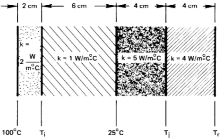
Calculateqand the temperature of the right-hand side of the wall.