UNIVERSIDADE DA BEIRA INTERIOR
Engenharia
Thermal Modelling and Experiments for Small
Satellites
Daniel Campanudo Carvalhais
Dissertação para obtenção do Grau de Mestre em
Engenharia Aeronáutica
(Ciclo de estudos integrado)
(Versão final após defesa)
Orientador: Prof. Doutor Francisco Miguel Ribeiro Proença Brójo
Orientador: Paulo Vasconcelos Figueiredo
Co-orientador: André Gomes da Costa Guerra
Co-orientador: Miguel Sousa Machado
Dedication
Acknowledgments
I would like to express my gratitude to my supervisor at UBI: Professor Francisco Brójo for all the help and for being always there for me, proving me the essential to conclude my experiments. Many thanks to my supervisor at CEiiA, Engineer Paulo Figueiredo. It was you who inspired me to complete this work, helping me and showing the right path to follow when I needed most. I always felt comfortable under your guidance. At the same time, I would like to thank CEiiA for giving me this opportunity to enrich me as a person and as a professional. Moreover, this gratitude includes CEiiA’s team for helping me during my experiments.
Thank you all whom helped me during this thesis, especially huge thanks to my girlfriend Inês and all my friends Lucas, Paco, José, Paulo, Oliveira, Luís, Ruizinho, Laudino, Kikões and Tiago. More than helping me you were always supportive in getting me out of my shell.
Desertuna. All the skills, lessons taught, adventures and stepped stages I will never forget and always carry in my heart. Our story is not fully written.
Last but not least, I would like to express my gratitude to my parents, Manuel and Maria, and my sister for the unconditional support and care during this journey.
Resumo
Tem havido um crescente interesse nas missões e na obtenção de dados através da utilização de CubeSats. Estes, devido à sua dimensão e baixo custo têm uma grande flexibilidade em acomodar diferentes cargas úteis. No entanto, novas missões com cargas úteis e componentes altamente sensíveis à temperatura, o aumento da dissipação de energia (pela miniaturização de componentes e sistemas eletrónicos) e superfícies irradiadoras reduzidas levam a possíveis problemas térmicos. Uma das causas para a falha de um satélite em órbita são os picos de tem-peratura sofridos durante um ciclo orbital completo. Portanto, o projeto e o teste adequados do sistema de controlo térmico devem ser realizados, de forma a garantir a fiabilidade do satélite antes do seu lançamento de modo a reduzir a possibilidade de falha.
O 3-AMADEUS é um CubeSat de uma unidade que está atualmente a ser desenvolvido numa parceria entre o CEiiA e a UBI. O propósito desta missão é demonstrar que um sistema de deter-minação e controlo de atitude exclusivamente magnético, pode ser capaz de fornecer atitude orbital de três eixos para os nanossatélites. O presente trabalho tem como objetivo efetuar análises térmicas ao 3-AMADEUS CubeSat para confirmar a sua sobrevivência assim que for colo-cado em órbita. Para isso, é necessário analisar os principais processos de transferência de calor num satélite, condução e radiação, de forma a validar as metodologias atualmente utilizadas para as análises térmicas. Assim, com o objetivo de desenvolver modelos térmicos com maior fiabilidade, foram realizadas duas experiências em vácuo.
O primeiro teste experimental consiste num estudo da troca de calor entre duas placas de alumínio através de radiação, usando uma lâmpada de infravermelhos como fonte de calor. Foram testadas três configurações de distância entre as placas e dois tipos de lâmpadas para comparação. Este teste simularia, por exemplo, a transmissão de calor entre diferentes compo-nentes dentro do satélite. Relativamente à condução, a maioria dos nano e microssatélites são compostos de PCBs empilhadas, mantidas juntas por espaçadores e varões roscados, conectados à estrutura principal. Esta é a principal forma de conduzir calor dos componentes para as super-fícies irradiadoras. Associada à interface entre a PCB e os espaçadores, existe uma resistência térmica que é um parâmetro desconhecido com grande impacto nas análises térmicas. Desta forma, foi realizado uma segunda experiência para estudar a resistência térmica de contacto (ou condutância) entre uma PCB e espaçadores.
Paralelamente, o software de elementos finitos (MSC Nastran) é usado para realizar um estudo numérico das mesmas experiências. Os resultados da distribuição de temperatura das soluções numéricas e experimentais foram então comparados e os resultados foram discutidos. Final-mente, com os resultados obtidos durante os testes foi realizada uma análise térmica em estado estacionário ao 3-AMADEUS CubeSat.
Palavras-chave
Análise térmica de CubeSat, Radiação térmica entre placas paralelas, condutância térmica en-tre contactos, resistência térmica em interfaces, validação do sistema de controlo térmico, contacto entre circuitos impressos e espaçadores
Abstract
There has been an increasing interest in CubeSat missions due to its small size, low cost and flexibility to accommodate different payloads. New missions with highly temperature sensitive payloads, increased power dissipation (by continuous miniaturization of electronic components and systems) and reduced radiating surfaces lead the thermal loads issues into a bigger chal-lenge. One of the causes of failure in a satellite in space is the temperature peaks suffered during a full orbital cycle. Therefore, proper thermal control system design and test should be performed to guarantee the reliability of a spacecraft prior to launch.
3-AMADEUS is a unity CubeSat currently being developed in a partnership between CEiiA and UBI. The purpose of this mission is to demonstrate that a attitude determiner and control sys-tem exclusively magnetic is able to provide a three axis orbital attitude for the nanosatellites. The present work aims to perform thermal analysis to 3-AMADEUS CubeSat in order to ensure its survival as soon as it is placed in orbit. Therefore, it is required the understand the main heat transfer processes within a satellite, conduction and radiation, in order to validate the current methodologies used for thermal analysis. Hence, with the purpose of developing thermal models with higher reliability, two experiments were devised to be performed in a vacuum environment. The first experimental test consists in a study of heat exchange between two aluminum plates through radiation, using an infrared lamp as a heat source. Three distance configurations be-tween plates and two lamp types were tested to comparison. This would emulate, for example, the heat transmission between different components within the satellite. Regarding the conduc-tion experiment, most nano and micro satellites are composed of stacked PCBs, held together by spacers and rods and linked to the main structure. This is the primary mean to conduct the heat from the different components to the external radiating surfaces. A high thermal resistance is associated with the interface between the PCB and the spacers, which is an unknown parameter with a high impact on the thermal analysis. Therefore, a second experiment is carried out to study thermal contact resistance (or conductance) between them.
In parallel, finite element software (MSC Nastran) is used to carry out a numerical study of the same experiments. The temperature distribution results of both numerical and experimental solutions were then compared, and the results were discussed. It was concluded that the re-sults obtained in both experiments, in general, presented a good agreement. Finally, with the results obtained in the numerical simulations and using the validated methodology, a steady state thermal analysis was performed to 3-AMADEUS.
Keywords
CubeSat Thermal Analysis, Thermal radiation between parallel plates, Thermal contact conduc-tance, Thermal contact resisconduc-tance, Thermal control system validation, interface between PCB and brass spacer
Contents
1 Introduction 1
1.1 Motivation . . . 1
1.2 Purpose and Contribution . . . 2
1.3 Context . . . 2
1.3.1 3-AMADEUS CubeSat Project . . . 3
1.4 Research and Objectives . . . 3
1.5 Thesis Outline . . . 4
2 Literature Review 5 2.1 Satellite History Overview . . . 5
2.2 Spacecraft Subsystems . . . 7
2.3 CubeSats . . . 7
2.4 Space Thermal Environment . . . 9
2.4.1 Direct Solar Radiation . . . 9
2.4.2 Earth Albedo . . . 10
2.4.3 Earth Infrared Radiation . . . 11
2.5 Thermal Control System . . . 11
2.5.1 Passive Thermal Control Systems . . . 12
2.5.2 Active Thermal Control Systems . . . 12
2.6 Thermal Verification Tests . . . 13
3 Heat Transfer and Thermal Analysis in CubeSats 15 3.1 Heat Transfer . . . 15
3.1.1 Conduction . . . 16
3.1.2 Radiation . . . 18
3.2 Numeric Heat Transfer Methods . . . 21
3.2.1 Finite Element Method (FEM) . . . 22
3.2.2 Boundary and Initial Conditions . . . 23
3.2.3 Linear Steady-State Heat Transfer Problem . . . 23
3.3 Thermal analysis of nano-satellites . . . 24
4 Experimental Study 27 4.1 Experimental Study Description . . . 27
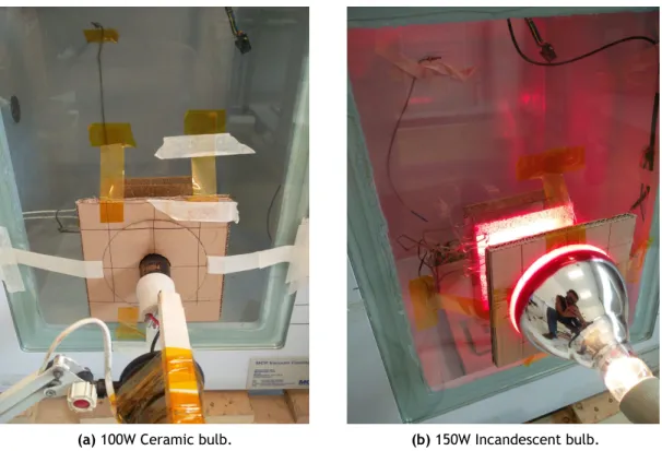
4.1.1 Radiation Experiment . . . 28
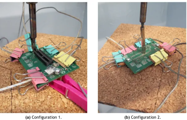
4.1.2 Thermal Contact Conductance Experiment . . . 29
4.2 Aluminum emissivity measure . . . 30
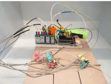
4.3 Data Acquisition System . . . 31
4.3.1 Calibration . . . 32
4.5 Experimental Results . . . 34
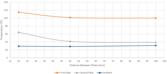
4.5.1 Radiative Parallel Plates . . . 34
4.5.2 Thermal Contact Conductance . . . 36
5 Numerical Study 39 5.1 Analytical Analysis . . . 39
5.2 Software Description . . . 40
5.3 Experiments Modeling, Meshing and Boundary Conditions . . . 41
5.3.1 Thermal Radiation Analysis . . . 42
5.3.2 Contact Conductance Analysis . . . 42
5.4 Mesh Convergence Study . . . 43
5.5 Results . . . 43
5.5.1 Thermal Radiation Analysis . . . 44
5.5.2 Contact Conductance Analysis . . . 47
6 Thermal validation of 3-AMADEUS CubeSat 49 6.1 3-AMADEUS Anatomy . . . 49 6.2 Thermal Requirements . . . 49 6.3 Simulation Cases . . . 50 6.3.1 Hot Case . . . 51 6.3.2 Cold Case . . . 51 6.4 Thermal Model . . . 51 6.4.1 PCB Thermal Conductivity . . . 52 6.4.2 Conductive Links . . . 53 6.5 Results . . . 54 7 Conclusions 57 7.1 Overview . . . 57
7.2 Constraints and Challenges Experienced . . . 58
7.3 Open points & Future Work . . . 59
Bibliography 61 A 65 B 66 B.1 Test Rigs . . . 66
C 68 C.1 Radiation experiment thermocouple readings over time . . . 68
D 70 D.1 Experiments Numerical Simulations . . . 70
E 71 E.1 CubeSat Model Details . . . 71
E.2 Environment Input Fluxes . . . 72
List of Figures
2.1 Satellite subsystems division. . . 7
2.2 CubeSats sizes from 1U to 16U. . . 8
2.3 CUTE-I satellite flight model . . . 8
2.4 Nanosatellite launches with forecasts for the next years. . . 9
2.5 Satellite thermal environment in Earth’s orbit. . . 9
2.6 CubeSat’s thermal vacuum testing. . . 13
2.7 Temperature definitions for thermal control system . . . 14
3.1 Thermal contact resistance . . . 17
3.2 Representation of the heat flow through rough contacting surfaces, with emphasis to the microscopic phenomena. . . 17
3.3 Absorption, reflection and transmission of a real body . . . 19
3.4 Radiative exchange between two area elements. . . 20
3.5 Radiation view factor for radiation between parallel plates. . . 20
3.6 Boundary conditions. . . 23
3.7 Heat flux across an insulated bar . . . 23
3.8 Flowchart of the design process and analysis of TCS. . . 25
4.1 Overview of test set-up in the thermal vacuum chamber and data acquisition system. 27 4.2 Radiation experimental test rig. . . 28
4.3 Radiation experiment test rig inside the vacuum chamber with both lamp config-urations. . . 29
4.4 Test set up schematics with the use of nylon washers. The numbers represent the location and position of the 5 thermocouples. . . 30
4.5 Experimental test rig inside the vacuum chamber with instrumentation. The ex-perimental rig is attached to the heat sink (aluminum plate covered by cork on the top). . . 31
4.6 Estimating the emissivity value by comparing the temperature measurement from thermocouple sensor with the value measure by the thermal camera. . . 31
4.7 Seebeck thermoelectric effect. . . 32
4.8 Data acquisition system assembly. Each thermocouple is connected to one amplifier. 33 4.9 Thermocouple calibration with two water points (a) hot bath, 100ºC and (b) cold bath, 0.0ºC. . . 33
4.10 Plotted experimental data from the Ceramic Bulb experiment for each separation distance. . . 35
4.11 Plotted experimental data from the Incandescent Bulb experiment for each sep-aration distance. . . 35
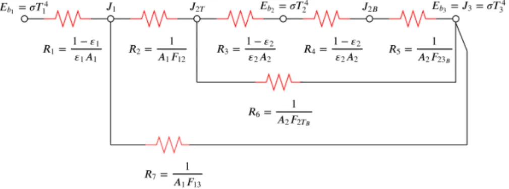
5.1 Radiation network for two parallel plates exchanging heat between them and an enclosure. . . 39
5.2 Process of FEM thermal analysis divided in pre-processing, solver and post
pro-cessing. . . 41
5.3 Thermal radiation between plates modeled in HyperMesh. Triangles represent the temperature constraints and the pyramids represent radiative elements (CHBDYE). 42 5.4 Thermal contact conductance experiments modeled in HyperMesh. (a) Top side of Test 2 and (b) Bottom side of Test 4. . . 43
5.5 Quad element mesh convergence. . . 44
5.6 Thermal distribution of Plate 2 at distance 3 from the first plate. . . 44
5.7 Temperature comparison between FEM analysis and Experiment 1 (Ceramic Bulb). 45 5.8 Temperature comparison between FEM analysis and Experiment 2 (Incandescent Bulb). . . 45
5.9 Model of the 100mm separation case. . . 47
5.10 Results obtained for both configurations with hc= 80.4mW/mm2K. . . . 47
6.1 3-AMADEUS concept structure and main subsystems. . . 49
6.2 Representation of the considered worst case cold and hot with an orbit with . . . 50
6.3 Comparison between CATIA 3D model and the 1D modeled rib in HyperMesh with the detailed 1D representation. . . 52
6.4 Meshed 3-AMADEUS CubeSat without solar panels. . . 54
6.5 Temperature ranges for hot and cold case along with operational temperatures. . 55
A.1 Surface characteristics by type of finish. . . 65
B.1 Test rig details without thermocouples. (a) Radiation experiment (b) Configura-tion 2 conductance experiment (c) Brass spacer detail used in conductance ex-periments. . . 66
B.2 Ceramic Bulb. . . 67
B.3 Incandescent bulb. . . 67
B.4 Vacuum chamber used to perform the experimental test. It provided the con-trolled environment desired. The convection heat transfer was minimized. . . . 67
C.1 Ceramic bulb, 20mm separation. . . 68
C.2 Ceramic bulb, 50mm separation. . . 68
C.3 Ceramic bulb, 100mm separation. . . 68
C.4 Incandescent bulb, 20mm separation. . . 69
C.5 Incandescent bulb, 50mm separation. . . 69
C.6 Incandescent bulb, 100mm separation. . . 69
D.1 Numerical results of power estimation analysis. . . 70
D.2 Thermal conductance model detail. . . 70
E.1 Satellite structure modeled in HyperMesh. . . 71
E.2 CubeSat stack connections detail. It is possible to identify CELAS2 elements used to simulate the thermal contact conductance. . . 71
E.3 RIB detail modelation. . . 72
E.4 Hot case results with solar panels. . . 73
E.5 Hot case results without solar panels. . . 73
E.6 Temperature distribution of OBC ABACUS, hot case. . . 74
List of Tables
1.1 Orbital details of 3-AMADEUS’s initial orbit . . . 3
2.1 Satellite classification in terms of deployed mass . . . 6
2.2 Satellite mission applications and common used orbits. . . 6
2.3 Summary of Heat Sources . . . 11
2.4 ECSS defined correlation success criteria. . . 13
4.1 Label of Figure 4.2. . . 28
4.2 Processed data of Ceramic Infrared Bulb experiment for the three different dis-tances between plates. . . 34
4.3 Processed data of Incandescent Bulb experiment for the three different distances between plates. . . 34
4.4 Experimental results of configuration 1. . . 36
4.5 Experimental results of configuration 2. . . 37
5.1 Error % between experimental and numerical Results (Ceramic and Incandescent Bulb, respectively). . . 45
5.2 Power estimation results for all test configurations. . . 46
5.3 Comparison between results obtained in experimental and simulations for both configurations. . . 48
6.1 Operational temperatures of 3-AMADEUS components and internal heat dissipation in both worst case scenarios. The orbit is considered at an inclination of i = 0. . 50
6.2 List of material thermal properties for 3-AMADEUS CubeSat. . . 53
E.1 Environment input loads used in the thermal model calculated for the orbit con-sidered. . . 72
Acronyms List
AU Astronomical Unit
CAD Computer Aided Design
CEiiA Centre of Engineering and Product Development COTS
Commercial-
off- the-shelf
ECSS European Cooperation for Space Standardization
ESA European Space Agency
FEM Finite Element Analysis
GEO Geostationary Earth Orbit
GPS Global Position System
HEO Highly Elliptical Orbit
IR Infrared
ISIS Innovative Solutions in Space
ISS International Space Agency
LEO Low Earth Orbit
LWR Long Wave Radiation
MEO Medium height Earth Orbit
MLI Multi Layer Insulation
NASTRAN Nasa STRuctural Analysis
OBC On Board Computer
PCB Printed Circuit Boards
PDE Partial Differential Equations
RMS Root Mean Square
TC Thermocouple
TCS Thermal Control System
TMM Thermal Mathematical Model
TVC Thermal Vacuum Cycling
Nomenclature
δ0 Gap thickness parameter
δU Internal Energy
˙
QPlanet Emitted heat by Earth ˙
QAlbedo Reflected solar abortion energy ˙
QSun Solar radiation absorbed
A Flat surface area
Aa, Ar apparent and real contact areas
D Distance between plates
E Modulus Elasticity
Eb Emissive power
F Force
Fij View factor between surface i and j
FSC−P View factor between the spacecraft and the planet
G Irradiation Gs Solar Constant H Microhardness hc Contact Conductance J Radiosity k Thermal Conductivity
ks Effective thermal conductivity
L Lenght
ms Effective absolute mean asperity slope
P Pressure
Q Rate of heat transfer
Q heat flow rate
Qexternal Environmental heat absorbed
Qinternal Power dissipated by internal components
Qout Heat rejected
Qradiated Heat emitted to space
r Specimen radius
Rj Thermal contact Resistance
T Temperature
Tm Interface temperature
W Work done by the system
Greek Letters α Absorptivity ϕ Zenith Angle ρ Reflectivity σ Stefan-Boltzmann Constant τ Transmissivity ε Emissivity Subscripts 1, 2 specimens 1 and 2 i, j specimens i and j
Chapter 1
Introduction
This chapter is devoted to the presentation of the motivation to develop accurate thermal analysis to satellites. The context in which this thesis is developed, is introduced as well as the 3-AMADEUS project. The purpose of solving the problem and the contributions to the scientific community to overcome the upcoming thermal problems associated to CubeSats are presented. The objectives of this work are introduced and finally the thesis structure is explained.
1.1
Motivation
Since the first satellite was put in orbit over 50 years ago, satellites have increased in size and weight and consequentially the cost to launch them into space increased as well [1]. However, small satellites more properly CubeSats, have gained a particular interest and are revolutionizing the future of spaceflight. Their small size and defined standards allow it to be a multi-purpose and low cost platform, flexible to accommodate different payloads and the ability to perform several missions.
However, once in orbit, these temperature sensitive components can suffer fatal failure. The satellite is exposed to intense periods of solar radiation and umbra during the orbital cycles. This results in critical temperature peaks which could be the cause of failure of the full system [2]. Furthermore, the heat produced inside the satellite by electronics must be conducted to the external faces to be rejected through radiation to the surrounding environment. There-fore, all components inside the satellite must be operated in a certain operational temperature range. In order to do so, a thermal control system design, analysis and testing is critical on satellite’s the development. The thermal analysis provide temperature distribution estimations which are used to guarantee that the thermal requirements are fulfilled and thus, confirming the reliability of the spacecraft prior to launch. Despite that, these analyses must be reliable and to make them so, is necessary to validate it through experimental tests.
It is necessary to understand how radiation is exchanged between surfaces in a vacuum environ-ment, considering the entire enclosure. Radiation exchange between surfaces is highly influ-enced by surface characteristics and geometry, orientation and separation distance, known as view factors. Numerical calculation of view factors is a key point for thermal radiation problems since the calculations can be very complex. On one hand software is fully capable of perform-ing these calculations, however error can be introduced derived approximations made. On the other hand, detailed analysis could be quite time consuming and a trade off must be searched. Another important parameter usually unknown is the high thermal contact resistance is asso-ciated to the contact between spacers and PCB’s. The heat flow path is important to control electronics temperature. Breaking this heat flow path could be dangerous and lead to
overheat-ing which could cause failure [3]. In past analysis a non measured value was used, rather it was used safety value, which gave temperatures different to those experienced in orbit. Therefore, estimating the thermal contact resistance between spacers and PCBs is a major challenge in thermal analysis of CubeSats.
Thermal contact conductance is influenced by several parameters and has been studied since 1960’s. Numerous expressions and correlations were made in a vacuum environment. However, almost all of these studies involved two generic mating solids with a known-constant pressure. As a result of the uncertainty of pressure and lack of description of the process, determining the thermal contact conductance becomes difficult. Therefore, it is essential to perform specific experiments to gain knowledge about the actual value in a specific contact such as the spacer-PCB interface.
1.2
Purpose and Contribution
In the early years of CubeSats, thermal analysis were rarely done and when performed, low fidelity models were used with unknown parameters and material properties. Additionally, experimental test and flight data correlation with thermal models was not done, preventing CubeSat developers from improving their modeling. Therefore, accurate and validated analysis must be performed to the thermal control system of satellites prior to launch to assess it. In the light of this matter, it is proposed test rigs construction for experimental radiation and thermal contact conductance studies. It is expected that the findings validate and improve the accuracy of thermal analysis for better prediction the spacecraft and subsystems temperatures. Thus, minimizing the risk of failure and loss of the spacecraft once in orbit.
To accomplish the main purpose, it is essential to fully understand the heat transfer methods, in particular thermal radiation and conduction between two contacting bodies. These mecha-nisms are studied analytically and numerically. Subsequently, the results obtained are used to validate the actual thermal control system of 3-AMADEUS, currently being developed at CEiiA and UBI.
Additionally, CEiiA is participating in several space related projects, the work presented in this thesis presents a important contribution for actual and future thermal analysis. Currently, CEiiA uses MSC Nastran to perform thermal analysis. Therefore, numeric methods must be understood and validated through experimental data. Considering the work presented, CEiiA will be able to use the knowledge acquired for current and future projects thermal analysis, such as small satellites or even a launcher for further analysis.
1.3
Context
The goal of this thesis is to gain confidence when performing thermal analysis to satellites. Thus, the ultimate work intents to validate the thermal control of the 3-AMADEUS CubeSat. Since repairs can be done in space, after the satellite’s launch, is crucial to validate t thermal control system. Thereby, it is assured that all the money invested in developing the satellite isn’t wasted in case of thermal failure. Therefore, reliable thermal analysis and methodologies
must be pursued.
1.3.1
3-AMADEUS CubeSat Project
The 3-AMADEUS(3 Axis Magnetic Attitude Demonstration Experiment for a Unit Spacecraft) is a 1U CubeSat currently under development in a collaboration by CEiiA and UBI. At this point, magnetic attitude determination and control devices are one of the cheapest, most reliable, small and lightweight attitude systems. However, they have limitations, in particular a rel-atively low accuracy (2º to 10º depending on disturbing torques acting on the satellite) and actuation capability requiring attitude sensors and actuators. Therefore, the mission objective is to demonstrate that a solely magnetic Attitude Determination and Control System might e capable of providing three-axis orbital attitude for Nanosatellites. The attitude information gathered during the whole orbit is sent and send it to earth at appropriate times.
The spacecraft’s orbit will be a 550 km approximately circular sun synchronous orbit. It will have the following orbit parameters:
Table 1.1: Orbital details of 3-AMADEUS’s initial orbit
Epoch 1 Jan 2020 Orbit Type LEO Altitude of Apogee / Perigee 550km
Eccentricity 0 Inclination 97.58º Argument of Perigee 0º
RAAN 270º
True Anomaly 0º Orbital Period 96 min
1.4
Research and Objectives
The main goal of this thesis is to gain confidence and understand the main heat transfer pro-cesses that occur in a satellite in order to perform accurate thermal analysis. The following objectives were defined for this research are summarized as follows:
• Review the main technologies used for thermal control of CubeSats;
• Gather the currently methodologies, both numerical and experimental, used to validate the thermal control system;
• Develop test rigs to investigate two important heat transfer processes that occur in a satellite, emulate the same experiments thereby validating the thermal analysis;
• Estimate the thermal contact conductance between spacers and PCBs through an indirect method;
• Analyze and validate the current thermal control system of 3-AMADEUS and provide sug-gestions if necessary;
• Create a methodology to perform thermal analysis in points which are difficult to calculate, such as contacts.
The objective of performing the experiments leads directly to the thermal analysis of the 3-AMADEUS CubeSat and validation of the thermal control system. The validated numerical anal-ysis will answer the question if whether or not the actual thermal control system is sufficient to survive the space thermal environment and provide insights where changes are needed.
1.5
Thesis Outline
This thesis is divided in seven chapters. The description of each chapter is mapped as follows:
Chapter 1 introduces the motivation to solve the research problem. It presents the purpose of
this work and the contribution to the scientific community. Lastly, the objectives expected to be achieved during this study are presented.
Chapter 2 starts with an introduction to the satellites history. The CubeSat concept and the
3-AMADEUS project are introduced. The spacecraft subsystems division is presented, which allow to introduce the thermal control system and continues with a description of the space environ-ment.
Chapter 3 presents the theoretical basics of heat conduction and thermal radiation necessary
to define the heat balance equations for the thermal modeling of satellites. The main theo-ries for thermal contact conductance estimation are presented. Finally, numeric heat transfer methods, the basics of FEM and the Software are introduced in this Chapter.
Chapter 4 describes both experimental tests performed and test rig development. Data
acqui-sition system assembly and test facility are described in this chapter. Material, schematics and procedure are explained in this chapter. The experimental results are presented and discussed.
Chapter 5 details the numeric analysis of the experimental tests performed. The modeling
steps and boundary conditions attributed are presented. Finally, the numerical results for both analysis are presented, compared with experimental data and discussed.
Chapter 6 characterizes 3-AMADEUS CubeSat and provides the steps taken to develop the
ther-mal model. The simulation cases, worst case scenarios, are formulated and described. Therther-mal analysis results are presented and conclusions made.
Chapter 7 recaps the work performed with a conclusion and achievements obtained.
Difficul-ties suffered performing the experiments are presented. Solutions to solve these difficulDifficul-ties are discussed.Finally open points and future work recommendations are provided.
Chapter 2
Literature Review
This chapter details the important role satellites play, being practically indispensable in all hu-manity activities such as scientific, telecommunications and Earth observation missions. The CubeSat concept is introduced, as well as the spacecraft subsystems division. Satellites have to survive extreme conditions. This allows to introduce the expected space environment, focusing on heat sources of a satellite in Earth’s orbit. Theory for environmental heat inputs calcula-tion is presented. Finally, thermal control system and main thermal control technologies are presented.
2.1
Satellite History Overview
Satellites can be split into natural and artificial and they can orbit either a planet or the sun. The moon is a good example of a natural satellite because it orbits Earth. Nowadays, artificial, or man-made machines launched to space are referred simply as ”satellites”. These machines are used primarily for communications, monitoring the weather and climate changes, for se-curity, for beaming television signal, for secure, robust three dimensional position (navigation) and technology demonstration. Nowadays, as we can’t live without computers, cars or mobile phones, we are fully dependent of satellites [4, 5].
The story of artificial satellites begins well before the first launch of a satellite. Isaac Newton was the first to imagine how a man-made satellite could orbit Earth in is Principia mathematica (1687). He theorized a cannon firing a ball from the top of a very high mountain that if fired with sufficient power would ’describe the same curve over and over’. However, he didn’t think of a satellite as a concept as we know today or it’s usefulness. At that time, there wasn’t a rocket powerful enough to put a satellite in orbit. Tsiolkovsky, in 1903, showed how satellites could be launched and calculated the required velocity in order to put a satellite into orbit. By the early twentieth century, the World Wars led to a period of high technological develop-ment, which started a race between the US and the Soviet Union to be seen which one would launch the first satellite. The Soviets won by launching Sputnik I in 1957, leading to the begging of Space Age. Since then, almost 8500 satellites were launched by more than 40 countries [6, 7]. Considering Portugal, PoSAT-1 was the first and only Portuguese satellite launched to space in 1993. It weights around 50kg and was used to test technology for future missions [8]. In 2020 is scheduled to launch Infante, the first developed and built satellite in Portugal. This will be a satellite mainly focused on maritime applications and will be developed by a consortium in which UBI and CEiiA are included. Furthermore, last year, Manuel Heitor, Portugal’s science and technology minister announced that fourteen enterprises were interested in building a space station in Azores. It’s expected that the first launches will take place in 2021. The main focus will be launching small satellites. Thus, if successful, this program will be a major step for
Portugal space industry, because it will attract companies dedicated to satellite development and therefore creating more workplaces [9].
Satellites can be classified by size, orbit, type of payload and therefore mission objective. They can vary from the size of a pickup truck to just the size of a small shoe box and have all shapes. Small satellites are defined as satellites weighing less than 500 kg. However, with the arrival of CubeSats and other very small satellites, it was necessary to create more terminology. The common classification by weigh is listed in Table 2.1.
Table 2.1: Satellite classification in terms of deployed mass and cost [10, 5].
Category Mass range (kg) Cost(M€) Large satellite >1000 >116 Medium-sized satellite 500 - 1000 29-116 Small Satellites Minisatellite 100 - 500 8-29 Microsatellite 10 - 100 1-8 Nanosatellite 1 - 10 0.1-1 Picosatellite 0.1 - 1 <0.1 Femtosatellite <0.1 <0.1
Besides the different size,satellites can be divided accordingly to their mission. The main type of missions include interplanetary spaceflight, military and intelligence, commercial, sci-ence and applications, technology demonstration and education. Table 2.2 presents some pay-load/mission types as well as commonly used orbits and examples of missions.
Table 2.2: Space mission applications, common used orbits and examples [1].
Mission Trajectory type Examples
Communications Geostationary for low latitudes, Molniya and Tundra for high latitudes (mainly Russia), Constellations of polar LEO satellites for global coverage
IntelSat Iridium Earth resources Polar LEO for global coverage SPOT
SeaSat
Weather Polar LEO, or geostationary TRMM
NOAA Navigation Inclined MEO for global coverage
GPS GLONASS Galileo (ESA) Astronomy LEO, HEO, GEO and ’orbits’ around Lagrange points Hubble
JWST Space environment Various, including HEO Polar SORCE Military Polar LEO for global coverage, but various DSP
MILSTAR
Technology demonstration Various CubeSats
Note: GEO: Geostationary Earth Orbit; HEO: Highly elliptical orbit; LEO: Low Earth Orbit; MEO: Medium height Earth Orbit.
The first satellite placed into orbit over 62 years ago was considered a ”small” satellite. Al-though the size and complexity of satellites have grown considerably since that time, ironically the space industry is returning and evolving to smaller satellites. CubeSats, in particular, have gained a unique interest by students interested in space science, technology and missions. Com-panies are also attracted by the CubeSat market, searching for more affordable alternatives [11].
2.2
Spacecraft Subsystems
Satellites system are divided in several subsystems as can be seen in Figure 2.1. This division reduces the interaction between subsystems and improve coordination between the different subsystem engineers [1]. This subsystems must provide the spacecraft ability to complete its mission. Therefore, the spacecraft must be able for example to point the payload in the right direction, change or correct the orbit, allow communications with the ground and energy man-agement [5].
Figure 2.1: Satellite subsystems division [1].
Although they are not directly connected between them, the design of each system or subsystem has direct impact and resources implication on the others [5]. Of all the subsystems the main focus of this thesis will be the thermal control system.
2.3
CubeSats
The term ”CubeSat” refers to a cube-shaped satellite measuring 100 mm × 100 mm × 100 mm and having a mass no greater than 1.33 kg. Prof. Jordi Puig-Suari at California Polytechnic State University and Prof. Bob Twiggs at Stanford University’s Space Systems Development Laboratory conceived the CubeSat standard in 1999 [12]. The original purpose of the project was to pro-vide affordable access to space for the university scientific community. The main idea was that a ”learn-by-doing” approach would provide students with hands-on experience in the field of spacecraft design and development [13]. However, in recent years a growing number of Cube-Sat missions indicate that the first CubeCube-Sats were almost as starting point for educational and technology demonstration. Thus, becoming a low-cost platform that could have science data return with high value and commercial revenue [14].
The specific standards for CubeSats help reduce the costs of technical developments and scien-tific investigations. These standardized aspects of CubeSats enable companies to mass-produce components and offer commercial-off-the-shelf parts (COTS). Therefore, the engineering and development of CubeSats becomes less costly than small satellites with customized design. Also, the costs associated to transporting and deploying them into space are reduced because of the standardized shape and size, and the possibility to launch several CubeSats with a single rocket
launch [15].
The standard size of a CubeSat is referred to 1U, with U representing a ”unit”. However, Cube-Sats can be aggregated to form a variety of sizes, such as the 1.5U, 2U, 3U and 6U [15]. Larger configurations are always in development as can be seen in Figure 2.2.
Figure 2.2: CubeSats sizes from 1U to 16U [16].
Figure 2.3: CUTE-I satellite flight model [17].
One of the first CubeSats launch to space was the CUbical Titech Engineering (CUTE-I) satellite (Figure 2.3), developed by the laboratory for Space Systems at the Tokyo Institute of Technol-ogy and launched on June 30, 2003. CUTE-I had three objectives: 1) demonstrate the ability to successfully download various satellite telemetry data in order to know the satellite condi-tions, 2) use the downloaded sensor data to calculate the satellite’s three-axis attitude and 3) demonstrate the effectiveness of a small deployment mechanism [17]. As can be seen in Figure 2.4, more than 1000 CubeSats were launched by 61 countries until this point and for the next 6 years over 3000 nanosats are expected to be launched [18].
The next years will show the evolution of the CubeSats applications. One example is the net-works of small satellites which distribute the tasks of a single common satellite. This network ideally would be autonomous, flexible, dynamically re-configurable, redundant and readily de-ployable [11].
Figure 2.4: Nanosatellite launches with forecasts for the next years [18].
2.4
Space Thermal Environment
Given the mission orbit parameters, the first step in any thermal analysis starts with the identi-fication of the sources of heat incident upon a satellite. The environment of a spacecraft is of extreme importance for the thermal management system. The main sources of environmental heating are direct solar radiation, Earth Albedo and Earth IR. These radiation fluxes depend on the orbital parameters, size, shape, view factors and surface properties of the spacecraft [19]. Furthermore, space can be considered as a heat sink at 3 K [20]. Figure 2.5 illustrates the main heat sources in space.
Figure 2.5: Satellite thermal environment in Earth’s orbit [21].
2.4.1
Direct Solar Radiation
the sun’s spectral distribution can be approximated as a blackbody at 5762 K [20] emitting pri-marily shortwave radiation. The value of the solar constant, the intensity of incident energy at 1 AU (Earth’s mean distance from the sun), is equal to GS = 1366.1W/m2. However, this value isn’t constant due to the the 11 year solar cycle and the Earth’s orbit. The first case has very little effect on the radiation emitted from the sun. The second case causes a variation of about 3.4%as a result of the eccentricity of the elliptical orbit which produces a geometrical varia-tion in the distance between the Earth and the Sun. Therefore, the electromagnetic radiavaria-tion values range from a minimum of 1321.6 W/m2at aphelion (summer solstice) and a maximum of
1412.9 W/m2 at perihelion (winter solstice) [19, 21, 20].
With a simple equation is possible to calculate the solar radiation absorptivity by a flat surface of area A, whose normal vector forms an angle θ with the solar rays:
˙
QSun= αGSAcosθ (2.1)
where α is the material solar absorptance of the surface and dependents on the surface’s finish [21].
2.4.2
Earth Albedo
The albedo of the Earth is the portion of the total incident solar radiation reflected by the planet to space. Its influence for thermal design is higher for low orbits. The value of Earth albedo vary with location and time. The main influences are the Earth’s topography and meteorological conditions. Other factors are the solar elevation angle and the spectral content of incident solar energy. As a result of the planet’s surface roughness albedo is assumed to be diffuse.
Generally, reflectivity increases with a increasing cloud coverage and a decreasing solar ele-vation angle, which varies during a day and seasonally. Additionally, varies with the Earth’s surface, being greater over continental regions than oceanic regions. In continental areas the albedo decreases with moisture. It can vary from small values over forests and higher values over desert areas. As for the ocean areas, since they absorb most of the incident radiation the albedo is between 0.05 and 0.1. Because of the high snow and ice coverage close the poles, associated with increasing cloud coverage and a decreasing solar elevation angle, albedo tend to increase with latitude [22]. The mean albedo value for Earth is assumed as 0.3, however, it must be used with care. A model to estimate the influence of latitude and longitude on albedo have been developed by the European Space Agency in [20].
When calculating the thermal loads on a satellite, it must taken in consideration that albedo loads must be used only when the portion of the planet seen by the spacecraft is sunlit. For simplified calculations, assuming the planet behaves as a reflecting sphere, the energy absorbed from albedo loads by an area A is
˙
QAlb= aGSAFSC−Pcosϕ, f or−
π
2 ≤ ϕ ≤
π
2 (2.2)
planet and ϕ the zenith angle.
2.4.3
Earth Infrared Radiation
A fraction of incident sunlight is absorbed by the Earth and its atmospheric gases. The Earth IR, or long wave radiation (LWR), is the emitted thermal radiation and it’s constant annually. Nevertheless, the intensity varies with time and from location to location on Earth’s surface. It depends on the local surface temperature and the cloud coverage. Warmer surface areas, such as deserts and tropical regions, will emit more radiation than colder areas. Cloud coverage will decrease the LWR, since lower clouds absorb radiation coming from the surface and the clouds top are at colder temperatures. In the case there are no clouds, the atmospheric temperature and moisture content become the main factors. The Earth IR unlike albedo has less variation across the globe [22].
The average temperature of the Earth’s surface is about 255 K and the emitted thermal radiation has a spectrum of a black body. This corresponds to an average flux of 230 W/m2. This value can
range from 150 W/m2to 350 W/m2for an orbiting spacecraft. Over ocean areas this flux is more
constant during the day than over desert areas [20]. With the planet’s average temperature, the flux incident on a spacecraft surface of area A can be obtained from:
˙
QP lanet= ϵAFSC−PσTP4 (2.3)
where ϵ is the infrared emissivity of the satellite surface and TP the temperature of the planet [21].
Earth albedo loads and infrared radiation are important for low orbits. However, for weather satellites in geostationary orbits these loads are insignificant, because of the low view factor. In Table 2.3 it is summarized the heat sources explained above.
Table 2.3: Summary of Heat Sources
Heat Source Value Direct Solar Radiation 1367 W/m2
Earth Albedo 0.3∗ 1367 W/m2 Earth IR 230 W/m2
2.5
Thermal Control System
The thermal control system must maintain a temperature stability using the less system re-sources possible. These limit temperatures are pre-defined upon the critical internal compo-nents. Examples of typical temperature requirements for main spacecraft components are -20 to +50 to electronic equipment and 0 to +20 for batteries. Controlling the components tem-perature not only ensures the reliability of the spacecraft, but also guarantees the optimum performance, preventing early degradation and success of the mission [5].
The hardware to control the temperature inside the satellite can be either active and/or passive. Each one is described in the following sections and examples are given.
2.5.1
Passive Thermal Control Systems
A passive thermal control technique is characterized by do not requiring input power nor moving parts for thermal regulation and are associated to low cost, volume, weigh and risk. Also, are proved to be reliable. They are the primarily technique for thermal control, relying on thermal conduction, radiation exchange and insulation systems [23]. Several options are readily avail-able to CubeSats. Some examples are summarized bellow.
Coatings and surface treatments are used to change optical properties of a surface. Thus, the thermal radiation environment is manipulated. The solar absortance and IR emittance can be varied according to the purpose needed and must be selected in order to achieve an energy balance at a desired temperature [19]. In small satellites the use of thermal tapes is easy to either apply or remove, and last longer than paints [24, 25].
Multi-layer insulation (MLI) or single-layer radiation barriers are used to insulate a satellite from radiation coming from the sun and reduces energy dissipation. MLI are composed of multiple layers of highly reflecting shields separated by non-metallic and low conductivity spacers in or-der to prevent contact between layers [19]. The use of MLI outside small satellites is uncommon due to the low efficiency in small areas, the outside surface being covered by solar cells and the necessity of rails clearance, due to the use of a deployer.
Thermal straps work with the same purpose of the heat pipes: transport thermal energy, pas-sively, from heat generator components to a thermal sink. They are usually manufactured in aluminum or copper, however recently efforts were put in developing more flexible thermal links using pyrolitic graphite and graphene sheets [23].
2.5.2
Active Thermal Control Systems
When CubeSats have high power demand, passive systems could be insufficient. Also, active systems are suited to applications where the spacecraft suffers large thermal fluctuations or seasonal variations, requiring thermal control for specialized payloads [23, 5]. However, the re-duced size of CubeSats, limits available options of active thermal control systems. It’s witnessed that the major quantity of active systems used in CubeSats consist in conventional technology used in larger satellites, which is size reduced in order to adapt to the small size of CubeSats.
Heaters consist in a electrical-resistance element between two layers of flexible electrically insulator material. Due to its flexibility they can be simply attached to any surface. The main disadvantage of heaters is the high energy consumption [19, 25].
Some payloads, such as high precision infrared sensors, imaging spectrometers, interferometers, require extremely low temperatures to operate. Temperatures less than 50K can be achieved through the use of cryocoolers [26].
2.6
Thermal Verification Tests
Thermal verification tests must be performed in order to validate the thermal model. The main objectives of thermal testing are: looking out for environmental stress, turn-on capabilities, survival demonstration, ETC [19]. The tests can be divided in two categories. One that confirm the validity of thermal control and other that endorse component’s integrity and workmanship [27]. These tests must be performed under a pressure of6 10−5hP aor less accordingly to ESA standards [28]
The validation of the thermal control system prior to launch is done through a thermal balance test. This test must be performed in controlled environment in specialized laboratories as can be . The need for this test is determined on a per project basis [29]. The objectives of perform-ing this test, as defined by the European Cooperation for Space Standardization (ECSS), are to provide data for verification of the numerical model in order to qualify the TCS, to demonstrate the appropriateness of the TCS design verify the performance of the TCS hardware, either ac-tive and/or passive, and to provide sensitivity data regarding certain components of the thermal control system [20].
ESA standards recommend performing two different steady-state cases and a transient case for components subjected to dynamic thermal behavior to validate the worst case scenarios [20].
(a) MinXSS-1 in Bemco-West themal
vacuum chamber [25]
(b) Thermal vacuum test set-up of STEP Cube Lab [30]
Figure 2.6: CubeSat’s thermal vacuum testing.
When the temperatures reached during the thermal balance test, are close enough to the pre-dicted in the thermal model, the test is considered successful. Typical values for temperature deviations are defined by the ECSS. As can be seen in Table 2.4, the temperature deviation for internal and external components must be lower than 5 and 10K respectively. For the temper-ature mean deviation a minimum of 25 measurements correlation is needed [20].
Table 2.4: ECSS defined correlation success criteria [31].
Temperature deviation for internal temperatures < 5K
Temperature deviation for external temperatures < 10K
Temperature mean deviation ±2K Temperature standard deviation < 3K, 1σ
A philosophy of safety margins applied to the calculated temperature ranges, in order to define qualification and acceptance tests, according to ESA Standards [20]. These margins are illus-trated in Figure 2.7.
Figure 2.7: Temperature definitions for thermal control system [31].
CubeSat developers do not need to perform the thermal vacuum cycling test (TVC) mandatorily. In this test, the spacecraft is exposed to a certain number of cycles, with pre-defined holding times and with given minimum and maximum temperatures. This test serves to check if there are any problems related to thermal stresses associated to temperature variation cycles on or-bit, by revealing any issues regarding malfunctioning or flawed components [15, 19].
Besides testing, a thermal vacuum bakeout is a requirement made by the launch providers to secure other missions in the same launcher. This is made to ensure proper outgassing of any possible contaminants of components before the actual launch [12]. Furthermore, it makes sure that optical and sensitive payloads aren’t contaminated. [15].
Chapter 3
Heat Transfer and Thermal Analysis in CubeSats
In this chapter, the basics of heat conduction and thermal radiation are explained. Its under-standing is vital to define the heat balance equations for the thermal modeling of satellites. Numeric heat transfer methods and the basics of FEM are introduced. A survey of the current methodologies used for CubeSat thermal analysis is performed. The theory presented will be necessary in the Chapters ahead.
3.1
Heat Transfer
Heat transfer is the science that deals with prediction of the rates at energy is transferred from one system to another because of a temperature difference. On the other hand, thermodynam-ics deals with equilibrium states and energy balance of all type of systems [27, 32]. For the thermal analysis of a spacecraft, the First Law of Thermodynamics states that energy can’t be created or destroyed, only transferred:
∆U = Q− W (3.1)
which simply states that the the rate of heat transfer to a system, Q, minus the amount of work done by the system, W , equals the variation of the internal energy, ∆U , of a closed system. The global thermal control of a spacecraft is achieved by balancing the heat rejected by the body against all the incident heat loads and the internal heat generated by the electronic subsystems (some of the power used by the electronics is released in the form of heat loads). From a generalized heat balance equation for conservation of energy:
Qout = Qin (3.2)
QRadiated= QExternal+ QInternal (3.3)
where QRadiatedis the heat emitted by the spacecraft to deep space, QExternalis the environ-mental heat absorbed, and QInternal is the power dissipation by the internal electronics. There are three mechanisms of heat transfer: convection, conduction and radiation. The last two are the main phenomena of heat transfer within a spacecraft in orbit. Convection is not observed in space because all systems of the spacecraft are in a vacuum environment. However, occurs for the most part on the ground, during ascent and in heat transfer from fluids contained
inside the satellite [27].
3.1.1
Conduction
Conduction is the process of heat transfer from particle to particle within a material or from two or more contact bodies. This indicates that in order for conduction to occur, a temperature gradient must present across the body. The process is given by Fourier’s Law :
qx=−kA
∂T
∂x (3.4)
where qxis the heat transfer rate, k is the thermal conductivity, A the cross sectional area per-pendicular to the direction of heat transfer and ∂T
∂x is the temperature gradient in the direction of the heat flow. The negative sign indicates heat flow from higher to lower temperatures [32].
Thermal conductivity is a material property that in most cases depends on the temperature. However, this value is almost constant within the temperatures observed in satellites. For spacecraft, the material properties and geometry of a system have an important role in the dissipation of heat generated by the electronics.
The Fourier equation ca be related to the Ohm’s law in electric-circuit theory as:
Heat f low = thermal potencial dif f erence
thermal resistance (3.5)
Thus, the electrical analogy can be used to solve complex problems, using both thermal resis-tances in parallel and in series.
3.1.1.1 Thermal Contact Conductance
When two materials are in physical contact with each other, illustrated in Figure 3.1a, heat is conducted from one face to the other and is subjected to a thermal contact resistance, defined as Rj= ∆Tj Q = T2A− T2B qAa (3.6) where the thermal contact resistance is defined as the ratio between the temperature drop across the interface and the total heat flux over the interface. The thermal contact resistance causes a drop in temperature over the interface, as can be seen in Figure 3.1b [19].
The main reason for the contact resistance, is the fact that surfaces, which seem to be smooth, on a microscopic level reveal asperity. This causes a reduction in the real contact area between the two contacting surfaces. The real contact area is just a small fraction of the apparent area [33]. The fraction between the actual and apparent area, Ar/Aa, depends on several parame-ters such as the surface roughness and waviness, surface hardness and contact pressure. Figure 3.2 shows the microscopic view of an interface.
(a) (b)
Figure 3.1: Thermal contact resistance: (a) interface between two materials ; (b) temperature profile of
a contact [32].
Figure 3.2: Representation of the heat flow through rough contacting surfaces, with emphasis to the
microscopic phenomena [34].
Contact conductance, more commonly used in literature, is defined as the inverse of the resis-tance
hj = 1
RjAa
(3.7) The heat transfer through the interface is considered to be the sum of three components. Con-tact conductance, hc, the conduction through the actual conCon-tacting points. Gap conductance,
hg, conduction through the interstitial medium. Radiative conductance, hr, thermal radiation between both surfaces. However, for bodies in space, which is a vacuum environment, the heat cannot be transferred through the medium. Furthermore, radiation can be neglected for most of space applications due to the low temperatures involved. Therefore, for the purpose of this thesis, the thermal joint conductance can be assumed to equal the contact conductance [19, 35]. Thermal contact conductance is affected by several factors, depending mainly on the two ma-terials in contact. The main parameters are listed below [19, 35].
• The thermal conductivity of the contacting materials; • The contact pressure;
• The surface roughness; • The surface hardness;
• The average temperature of the junction.
The engineer must be cautious when choosing a model to use in satellite design calculations. Assumptions made for each model should be taken in account [19].
3.1.1.2 Related Work
Several studies were made to estimate thermal contact conductance in common CubeSat stacks. Berggren in 2015 performed experiments to measure the thermal conductance between a PCB and the mounting screw associated to a sleeve. The mean value obtained for the conductance was Gmean = 0.0160 W/K which correlated well with the theoretical calculated value [36]. Flecht in 2016, compared the results from simulations with measurements of an actual model. Finally, the contact conductance in the thermal model are adjusted to match the engineering model [37].
Recently, Hager [38] performed experiments with eight different configurations in vacuum. For aluminum spacers without washers the contact resistances was found to be ranging from 33.500 to 107.000 W/m2K.
3.1.2
Radiation
Although heat transfer within a satellite can occur by radiation and conduction, the only means by which the vehicle can exchange heat with its environment is by radiation. Mechanisms to con-trol temperature, either active or passive, must reject heat by radiation to space. Therefore, an accurate analysis of the radiant heat transfer is of extreme importance for better prediction of the spacecraft and subsystems temperatures.
All bodies emit and absorb electromagnetic energy when their temperature is above absolute zero. This process is known as thermal radiation, which is ruled by the amount of radiant energy emitted by a blackbody per unit time and per uni area Eb, also known as Stefan-Boltzman law, which states that total energy emitted is proportional to absolute temperature to the fourth power:
Eb = σT4 (3.8)
where T is the body’s temperature in Kelvin ans σ is the Stefan-Boltzmann constant, which has the value σ = 5.669× 10⁻⁸W/m2· K4. Eb is in watts per square meter and is named emissive
power of a blackbody [32].
3.1.2.1 Radiation Properties
Equation 3.8 have been developed for a blackbody which is an idealized object that appear black to the eye and absorbs and emits all incident radiation. However, no object is a perfect black body, real bodies absorb, reflect and transmit incident, as shown in Figure 3.3. We define absorptivity, reflectivity and transmissivity as:
Absorptivity α =
(
amount of absorbed radiation total incident radiation
)
,
Ref lectivity ρ =
(
amount of ref lected radiation total incident radiantion
)
,
T ransmissivity τ =
(
amount of transmitted radiation total incident radiation
)
,
Therefore, from the energy balance, the sum of these properties must be unity:
α + ρ + τ = 1 (3.9)
Furthermore, for almost all solid objects that are opaque, no thermal radiation gets transmitted through, τ = 0. Thus, α + ρ = 1 [39].
Figure 3.3: Absorption, reflection and transmission of a real body [32].
As stated before, real objects have lower emissivities than ideal black bodies. The emissivity is a function of the wavelength, the surface’s temperature and surface roughness. However, for most of the engineering applications, emissivity assumes typical values shown in literature [32]. Figure A.1 in Appendix A shows surface characteristics of several materials, paints and coatings commonly used in satellites.
The spectral, hemispherical emittance, compare the real spectral emissive power with the spec-tral emissive power of a black body surface and is defined as
ϵλ(T, λ) = Eλ(T, λ)
Ebλ(T, λ)
(3.10) For a blackbody, the emissivity is ϵ = 1 and for a real body 0 < ϵ < 1. So, the total emissive power of a real object becomes dependent on the emissivity:
E = ϵσT4 (3.11)
3.1.2.2 View Factors
energy exchange between two surfaces must be considered and analyzed. The view factor, or shape factor, from a surface m to a surface n is denoted by Fm→n and is defined as the fraction of the radiation leaving surface m that strikes surface n [32]. The view factors only depend on the geometry, size, orientation and distance between the surfaces. Considering two differential areas as shown in Figure 3.4 it’s possible to determine the differential view factor between them by:
dFdA1→dA2=
cosθ1cosθ2
πr2 dA2 (3.12)
where θ is the angle measured between a normal to the surface and the line that connects them
r. Integrating over two areas, A1 and A2, the view factor between two diffuse finite areas is
defined as: FdA1→dA2= 1 A1 ∫ A2 ∫ A1 cosθ1cosθ2 πr2 dA1dA2 (3.13)
An important property of equation 3.13 is the reciprocity relation which is stated mathematically by:
AiFij = AjFji (3.14)
Considering an enclosure, the general relation states that the sum of all view factors must be unity. For an enclosure with n surfaces the general relation is:
n ∑ j=1
Fij = 1.0 (3.15)
View factors can be calculated using analysis, numerical methods and analogy. The calculation presented is not practical, because even for simple geometries the integrations can be very difficult and complex. For the purpose of this thesis and for common geometries, such as that found in CubeSats, view factors are given in analytical, graphical and tabular form in several publications [40].
Figure 3.4: Radiative exchange between two area
elements [32].
Figure 3.5: Radiation view factor for radiation
3.1.2.3 Radiative Exchange Between Surfaces
For the purpose of this thesis, surfaces are assumed to be, diffuse and isothermal, in order to simplify the analysis and because nonblack bodies are involved [32]. Under these conditions and since transmissivity is assumed to be zero ϵ = ϵλ= αλ= α = 1− ρ. The total heat flux leaving a surface per unit time and per unit area is
J = ϵEb+ ρG (3.16)
where J is the radiosity and G is the irradiation, which is the total amount of energy incident upon a surface. By using the concept of gray and diffuse surface, radiosity becomes
J = ϵEb+ (1− ϵ)G (3.17)
Solving for G in terms of J, the net energy leaving a surface is given by
q = J− G A = Eb− J 1− ϵ ϵA (3.18)
where the numerator is considered as a potential difference, while the denominator is an oppo-sition to heat transfer. This interpretation allows the radiation analysis by the network method originated by Oppenheim [41]. Considering the heat exchange between two surfaces, illustrated in Figure 3.4, the net interchange between the two surfaces is
q1−2= J1A1F12− J2A2F21 (3.19) Analytically the view factors for parallel plates (Figure 3.5) are given by:
F1−2 = ( 2 πxy ) { ln [ 1 + y2 1 + x2+ y2 ]1/2 + x(1 + y2)1/2tan−1 [ x (1 + y2)1/2 ] + y(1 + x2)1/2tan−1 [ y (1 + x2)1/2 ]
−x tan−1x−y tan−1y }
(3.20) Other problems such as the three-body or the case of two surfaces enclosed can be solved by this method and are also important for this analysis [32].
3.2
Numeric Heat Transfer Methods
There are three methods to solve any engineering problem, the analytical, numerical and ex-perimental methods [42].
Experimental investigation involves the construction of full-scale model, used to get actual tem-perature measurements. This method is expensive and slow, since it requires at least 3 to 5
measurements.
Analytical methods using the conservation of energy principle as differential equations attempt to predict temperatures, solving using initial and boundary conditions. This method is only ap-plicable to simple cases of geometry, loading and boundary conditions.
Numerical methods attempt to predict/approximate the satellite’s temperature. This method subdivides the satellite into nodes or elements that are connected by conduction and radia-tion. Therefore, a numerical solution enables the determination of temperature only at discrete points.
At an early stage of design of a satellite, experimental methods are extremely expensive and time consuming. Besides that, the number of different material properties and other nonuni-formities would require immeasurable number of equations. Thus finding analytical expressions for temperature is generally not possible due to the complexity of the geometry and bondary conditions [43]. Therefore, computational methods are preferred, even less precise (approxi-mate values).
Among different methods of analysis, the finite element method is a very accepted and com-monly used method for thermal analysis. In this thesis, a finite element software is used. Therefore, only finite element method will be explored.
3.2.1
Finite Element Method (FEM)
The finite element method is a numerical mean to determine approximate solutions for partial differential equations (PDE) on a defined domain (W) [42]. Finite element consists of domain discretization into interconnected finite elements to create a thermal model. Thus, in each ele-ment the governing equation is approximated by any of the traditional variational methods [44]. A numerical model for satellite heat transfer starts with the definition of the physical problem. Besides this, the model can be divided into the discretization of the domain and the discrete approximation of the partial differential equations (PDE). Lastly, combining both, the numerical solution is obtained [43].
The basis for thermal analysis is the heat balance equation, which is based on the principle of energy conservation [43]. The heat balance equation expressed in Cartesian coordinates is given by ρcp ∂T ∂t = ∂ ∂x ( kxx ∂T ∂x ) + ∂ ∂y ( kyy ∂T ∂y ) + ∂ ∂z ( kzz ∂T ∂z ) + Q (3.21)
where the thermal conductivity, k, can be expressed as
k = kxx kxy kxz kyx kyy kyz kzx kzy kzz
directional variation in thermal conductivity.
3.2.2
Boundary and Initial Conditions
Before stating any analysis it’s necessary to state appropriate boundary and initial conditions. Thus, a solution for the heat conduction equation is possible. The boundary conditions can be divided in two types or a combination of both, as can be seen in Figure 3.6. The first, the
Dirichletcondition, in which the temperature on the boundaries is known and/or the N ewman condition, in which the heat flux is imposed [43].
Figure 3.6: Boundary conditions.
The insulated, or adiabatic and the symmetry conditions are obtained with ¯q = 0[43].
3.2.3
Linear Steady-State Heat Transfer Problem
In steady state calculations, the heat flux entering the satellite and the heat flux leaving are constant. Furthermore, material properties such as the conductivity are linear.
Figure 3.7: Heat flux across an insulated bar.
A simple heat conduction example in a laterally insulated uniform bar with a cross sectional area A and thermal conductivity k is shown in figure. Considering the Fourier heat conduction equation and the boundary conditions, the heat balance equation at the nodes are [45]:
Node 1: Q = kA ( T1− T2 L1 ) = kA L1 T1− kA L1 T2 (3.22) Node 2: Q = kA ( T2− T1 L2 ) = kA L2 T2−kA L2 T1 (3.23)
The above equations can be rewritten in matrix form as: kA L1 −kA L1 −kA L2 kA L2 { T1 T2 } = { Q1 Q2 } (3.24)
![Figure 2.4: Nanosatellite launches with forecasts for the next years [18].](https://thumb-eu.123doks.com/thumbv2/123dok_br/19174045.942425/31.892.215.726.106.421/figure-nanosatellite-launches-forecasts-years.webp)
![Figure 2.7: Temperature definitions for thermal control system [31].](https://thumb-eu.123doks.com/thumbv2/123dok_br/19174045.942425/36.892.143.710.208.474/figure-temperature-definitions-thermal-control.webp)
![Figure 3.1: Thermal contact resistance: (a) interface between two materials ; (b) temperature profile of a contact [32].](https://thumb-eu.123doks.com/thumbv2/123dok_br/19174045.942425/39.892.176.761.117.312/figure-thermal-contact-resistance-interface-materials-temperature-profile.webp)