www.nat-hazards-earth-syst-sci.net/11/2965/2011/ doi:10.5194/nhess-11-2965-2011
© Author(s) 2011. CC Attribution 3.0 License.
and Earth
System Sciences
The Henetus wave forecast system in the Adriatic Sea
L. Bertotti1, P. Canestrelli2, L. Cavaleri11, F. Pastore2, and L. Zampato2
1Institute of Marine Sciences – CNR, Venice, Italy
2Istituzione Centro Previsioni e Segnalazioni Maree, Venice, Italy
Received: 14 January 2011 – Revised: 9 May 2011 – Accepted: 27 June 2011 – Published: 7 November 2011
Abstract. We describe the Henetus wave forecast system in the Adriatic Sea. Operational since 1996, the system is con-tinuously upgraded, especially through the correction of the input ECMWF wind fields. As these fields are of progres-sively improved quality with the increasing resolution of the meteorological model, the correction needs to be correspond-ingly updated. This ensures a practically constant quality of the Henetus results in the Adriatic Sea since 1996. After suitable and extended validation of the quality of the results at different forecast ranges, the operational range has been recently extended to five days. The Henetus results are used also to improve the tidal forecast on the Venetian coasts and the Venice lagoon, particularly during the most severe events. Extensive statistics on the model performance are provided, both as analysis and forecast, by comparing the model results versus both satellite and buoy data.
1 Introduction
There is an obvious need for reliable forecasts of the wind wave conditions. In this paper we analyse the characteristics and the quality of such a forecast in the Adriatic Sea. This, with a wider perspective, can be considered as a typical ex-ample of inner and enclosed sea. In this case the situation can be, and frequently is, much different from the one present in the oceans and, although at a different level, in the Mediter-ranean Sea. On one hand, on the open space of the oceans, without any influence by the continents and their orography, the evolution of a meteorological system is intrinsically more predictable.
As an example, the 24-h forecast of the European Centre for Medium-Range Weather Forecasts (ECMWF, Reading,
Correspondence to:L. Bertotti ([email protected])
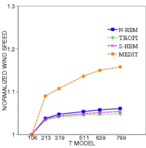
UK) has, at least in certain areas, a quality similar and of-ten superior to the analysis. The quality shows only minor decreases when moving to the 48- and 72-h forecasts (e.g. Bidlot et al., 2002; Richardson et al., 2010). However, the situation changes when we move to inner seas. All this is quite clear in Fig. 1, showing the progressive improvement of the ECMWF forecasts when we increase the resolution of the meteorological model. Note that, when using the T799 res-olution, i.e. the operational one till January 2010, the results do not improve further with resolution, a strong indication that in the oceans the model is close to the ideal solution. On the contrary, in the Mediterranean Sea the model wind speeds still increase with resolution, suggesting that we are still far from the ideal results.
The difficulties increase when we move to even smaller basins. For instance, in the oceans a small shift of the po-sition of a pressure minimum does not affect appreciably the overall structure of a storm. On the contrary, in a basin of limited dimensions a similar shift may lead to a drastic change of the local meteorological, hence oceanographic, situation. If, on top of this, we consider the influence of orography, we see at once that forecasting wind and waves in a small size basin, especially if surrounded by mountain ridges, may indeed be problematic. However, this is the sit-uation of the Adriatic Sea, a clear example of how difficult good quality long term forecasts can be.
In this paper we describe a wind and wave forecast system in the Adriatic Sea based on a combination of rigorous phys-ical approach and objective empirism, a combination that leads, as we will see, to very good results.
Fig. 1.Variability of the sea surface wind fields as a function of the resolution of the ECMWF meteorological model (after Cavaleri and Bertotti, 2006).
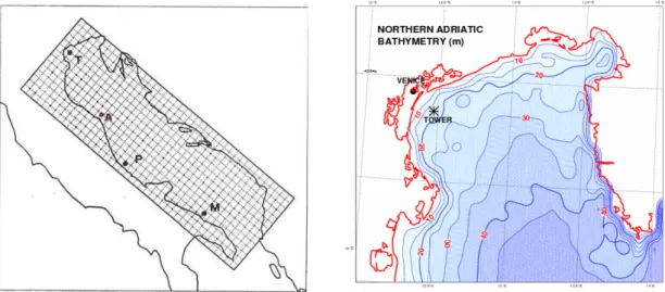
Fig. 2.The oceanographic tower of ISMAR in the northern Adriatic Sea, 15 km offshore the Venice coastline. Right panel: the tower (second floor, +7 m a.m.s.l.) after the storm of 22 December 1979. The position of the tower is shown in Fig. 3.
the coast that takes place when storm waves run directly to-wards it. Ignored for quite a while, this information became abruptly evident after the big storm of 22 December 1979 that led to one of the worst floods of the town. It took a while to digest this information and its implications, also because the tide forecast models, naturally tuned to the data of the past, seemed to include implicitly this wave effect. The rea-sons why this is not the case will be described in Sect. 8. For the time being it is sufficient to specify that wave information is necessary for tidal forecast.
Henetus is not the oldest wave forecast system acting in the Adriatic. ECMWF started its Mediterranean, hence also in the Adriatic, forecast in July 1992. However, the meteoro-logical model that provides the driving wind for wave fore-cast was and is necessarily global. Therefore it could not, especially at the time, have a resolution capable to describe the wind with the necessary accuracy. Besides, following the
progressive increase of computer power, the spatial resolu-tion of the ECMWF meteorological model has been chang-ing in time. So the resolution has moved from T213 (95 km) to T319 (60 km), T511 (40 km), T799 (25 km), and T1279 (16 km), the last one in January of 2010. Also, the resolution of the wave forecast in the Mediterranean has changed, pass-ing from the initial 0.5◦
to 0.25◦
, and finally to the present 0.1◦
. All this implies that the corresponding time series at the various locations are not homogeneous and, in any case underestimated, more so in the early years, both as significant wave height and wave period. Cavaleri and Bertotti (2006) provide a clear idea of the situation. This was also the reason why, because of both scientific and management reasons of the activities on the oceanographic tower of the institute (see Fig. 2), ISMAR decided since 1996 to run its own wave fore-cast system. Since the start, it was indeed based on the wind fields produced by ECMWF, but suitably corrected to take into account their underestimate (more about this in Sect. 3), in so doing avoiding, to a large extent, the non-homogeneity of the original fields.
It is correct to specify that there are several other fore-cast systems in the Mediterranean and, for most of them, also in the Adriatic. The mandatory example is NETTUNO (see Bertotti et al., 2010), a combined product of the Centro Nazionale di Meteorologia e Climatologia Aeronautica (CN-MCA) of the Italian Meteorological Service of Italian Air-Force and of the Institute of Marine Sciences (ISMAR) of the Italian National Research Council. This system, driven by the surface winds out of the high resolution COSMO-ME meteorological model (Bonavita and Torrisi, 2005), works with a 0.05 degree resolution and (see Bertotti et al., 2010) provides what are probably the best results presently avail-able in the Mediterranean Sea. Another system worthwhile mentioning is MEDITARE (see Valentini et al., 2007), op-erational at ARPA-EMR. Both these systems do not extend much in the past.
For several reasons it is clearly important to have avail-able long time series with a resolution capavail-able to ensure high quality results. This is hardly possible with a reanalysis (see, e.g., Lionello, 2005). The system we describe, named Hene-tus, has been operational with a similar operational structure since the Spring of 1996. Hence, it provides 14 yr time series of detailed wave information on the whole Adriatic concern-ing both analysis and forecast.
Fig. 3.Left panel: geometry of the Adriatic Sea and location of the ISMAR oceanographic tower (see Fig. 2), and the A=Ancona, P=Pescara, M=Monopoli wave measuring buoys. Right panel: bathymetry of the northern part of the basin. The grid in the left panel shows the field orientation in Fig. 4.
2 The Adriatic Sea
The geometry of the basin, enclosed between Italy and the Balcanic countries, is shown in Fig. 3. The Adriatic is about 750 km long and 200 km wide, practically closed, with only a limited connection, the Otranto strait, at its southern end with the Ionian, hence Mediterranean, Sea. The depth of the basin is rather limited in its northern part, with the bottom slowly sloping down (1/1000) from the coast. South of An-cona (point A in the figure), the bottom deepens suddenly, and from there on, for any wave study deep water conditions can be assumed.
The basin is surrounded by mountains, the Dinaric Alps to the east and the Apennines on the Italian side. The only flat borders are the southernmost part of the Italian coastline and the Po valley to the north-west, then enclosed by the Alps. Two typical wind systems dominate the meteorological situ-ation, bora and sirocco. They blow, respectively, from north-east and south-north-east, with quite different characteristics. Bora is a violent, often cold and turbulent, wind that, also because of a limited fetch, leads to young, steep and frequently break-ing waves. On the contrary sirocco blows along the main long axis of the basin. It does not reach the speed of bora, but, because of the long fetch, it may lead to the highest and longest waves in the Adriatic Sea. A more thorough discus-sion on the characteristics of the basin is given by Cavaleri et al. (1991) and Cavaleri (2000).
3 The meteorological and wave models
Any wave forecast system depends heavily on the accuracy of the driving wind fields. The high sensitivity of the result-ing waves to also limited variations of the input meteorologi-cal information makes it mandatory to have at one’s disposal a reliable source of wind data.
The Henetus system uses as input information the anal-ysis and forecast (see next section) wind fields produced by ECMWF. This uses a spectral model, the spatial fields of the various meteorological parameters being represented as two-dimensional spectral series. Starting January 2010, the series are truncated at T1279. This corresponds to a 16 km spatial resolution. The advection is evaluated with a semi-Lagrangian scheme, while the physics is dealt with on a reduced Gaussian grid. Wave models are convention-ally driven by the 10 m wind, obtained as a postproduct using a boundary layer model applied at the lowest level of the meteorological model. A compact description of the ECMWF model is provided by Simmons et al. (1995), Simmons and Hollingsworth (2002), Simmons (2006), and Palmer et al. (2007). On a global scale, repetitive statistics have shown that the ECMWF products are, and have been for a long while, the best ones in the world. However, as we mentioned in the Introduction, the quality decreases when we move to the inner seas, and in particular in the Adriatic.
Fig. 4. Wind and wave fields in the Adriatic Sea at 12:00 UTC, 10 March 2010. Arrows show the mean wind and wave directions, respectively, with length proportional to wind speed and significant wave height. The isolines are traced at 4 m s−1and 1 m intervals.
For a more compact plot the orientation is the one shown in Fig. 3.
essential scalar and vector parameters, i.e. significant wave heightHs, mean and peak periodTm,Tp, and mean direction
θm. In Henetus, the model has been recently implemented
on a geographical grid with 1/12 degree resolution (about 9×7 km in the Adriatic) using 30 frequencies (f1=0.05 Hz,
fn+1=1.1×fn)and 24 uniformly spaced directions. Note
that the grid in Fig. 3, clearly rotated with respect to geo-graphical coordinates, is shown only for the correspondence with the ones in Fig. 4.
Because the ECMWF wind is underestimated in the Adri-atic (Cavaleri and Bertotti, 2004), the derived wave heights would be similarly, or even more strongly, underestimated. Indeed, this is the case with the local ECMWF wave forecast. However, long term testing in the various meteorological sit-uations (see Cavaleri and Bertotti, 1997, 2006) has clearly shown that the geometrical structure of the fields is gener-ally correct (safe for a few details related to the local orogra-phy), the problem being only a reduction of the wind speeds with respect to the ground truth. Cavaleri and Bertotti (1997, 2006) have shown that increasing the ECMWF wind speeds by a given percentage brings both wind and wave results very close to the truth. However, the underestimate is related to the resolution of the meteorological model. Because this has been changing in time, it also has the necessary correction coefficient passing from 1.5 (T213 and T319, 1991–2000, using the same Gaussian grid) to 1.35 (T511, 2000–2006), to 1.26 (T799, 2006–2010), and to 1.20 for T1279 (since Jan-uary 2010). Before being operational, each new resolution is duly tested for a period between 6 and 12 months. During this period both the systems, the previous and the new one, have been running in parallel. This allows a new calibration
of the wind correction coefficient in the Adriatic Sea before the new system becomes operational, and therefore the avail-ability out of Henetus of a consistent sequence of wave fields of practically uniform quality.
4 The operational procedure
The Henetus wave forecast system operates on a daily ba-sis with a 120 h forecast range. At ICPSM the ECMWF wind data is part of the input information to the statistical storm surge forecast system (Canestrelli and Moretti, 2004; Canestrelli and Zampato, 2005; Bajo et al., 2007). The most recent version of the hydrodynamic model SHYFEM, oper-ational at ICPSM (Bajo and Umgiesser, 2010), is driven by the corrected wind (see previous section). At the same time the wind data are used to drive the WAM model, operational at ISMAR, to produce a five day wave forecast. The results, e.g. maps of the distribution of significant wave heights in the northern Adriatic (see the following section), are then passed to ICPSM and made available on the two websites www.comune.venezia.it/maree and www.ismar.cnr.it.
The structure of operations at ISMAR is as follows. At day D the system receives the information on the wind fields of the last 24 h (analysis) and for the next 120 ones (forecast). Based on this, and granted the cited correction of the wind speeds, WAM derives the corresponding wave conditions. These results are available after about 20 min and passed immediately to ICPSM. For logistical reasons this happens around 02:00 UTC. The day after, D+1, the procedure is re-peated, with the model starting from the analysis of day D to produce the D+1 analysis and the following five day forecast. Six independent time series are therefore available for later inspection of the quality of the results: the wind and wave analysis, and also the corresponding forecasts with range one day (F1, 0–24 h), two days (F2, 24–48), three days (F3, 48– 72), four days (F4, 72–96), and five days (F5, 96–120). The wave fields are available at three hour intervals, and concern, on each grid point, the integrated parametersHs,Tm,Tp, and
θm.
5 Results
Table 1.Statistics for the comparison of the significant wave height in the Adriatic Sea out of the ENVISAT altimeter and the corresponding model data. The considered period is 2005–2010. The results are shown for the overall period and for each single year. The mean satellite value is shown. The comparison is model vs. altimeter. Values are in metre. The scatter index is the ratio between the mean square error and the mean value.
overall 2005 2006 2007 2008 2009 2010
mean 0.98 1.00 0.98 0.94 0.96 0.99 0.98 best-fit slope 0.99 1.01 0.95 0.99 1.06 0.97 1.00 bias −0.09 −0.10 −0.14 −0.10 −0.06 −0.13 −0.03 scatter index 0.37 0.38 0.34 0.37 0.39 0.35 0.36
Correspondingly, after an extensive sirocco storm it is com-mon to see, for instance at the ISMAR oceanographic tower (see Figs. 2 and 3 for its position), swell arriving for at least one day with progressively decreasing wave period (shorter waves have a lower group speed).
Within the coherence between wind and waves in Fig. 4, note the more regular structure of the wave field. This is because waves are an integrated effect, in space and time, of the driving winds. As such, as a rule they do no display the possible strong spatial gradients that sometimes, e.g. the cold fronts, characterise the wind fields.
Figure 5 shows, at 24 h interval, one analysis field in the northern Adriatic, and the associated 24, 48, 72, 96, 120 h forecasts. We can clearly see how the limited response time of the basin may imply quite different wave conditions from one day to the next.
Beside having at disposal a synoptic view of the situation, it is clearly of interest to know, possibly in advance, the evo-lution of the conditions at a specific position. As a matter of fact, one of the original reasons to start wave forecast in the Adriatic was the logistics of the activities related to the oceanographic tower. Its position is also of direct interest to ICPSM as it represents the wave conditions just in front of the Venice littoral, facing the three inlets to the lagoon (see the Introduction). One example of analysis and follow-ing forecast is given in Fig. 6, where we see the estimated (analysis) and expected conditions (wind and waves) for the next 120 h. Please note that, contrarily to the meteorological convention, in the figure the wind is shown as flow direc-tion. Apart from the physics of the processes involved (en-ergy moves in the wind flow direction), this makes easier the comparison in the figure between wind and wave directions.
6 Comparison with the available measurements
The validation of the wave model results is done using the data available at the oceanographic tower (Fig. 2); at the wave measuring buoys of the Italian network RON (De Boni et al., 1993; see also www.telemisura.it), whose position in front of respectively Ancona, Pescara, and Monopoli is shown in Fig. 3; and from altimeters. The model data has been co-located with the measured data using a bi-linear
in-Table 2. As Table 1, but the statistics are now with reference to the data of the wave measuring buoys. See Fig. 3 for their position. Given the irregular availability of the buoy data, the statistics are provided only for the whole period.
Ancona Pescara Monopoli
mean 0.69 0.67 0.72 best-fit slope 1.03 1.02 1.19 bias 0.01 0.04 0.15 scatter index 0.32 0.38 0.41
terpolation in space for the tower and the buoys, and also a time interpolation for the altimeter data.
It is convenient to begin with a synoptic view of the qual-ity of the results. Figure 7 shows the ground traces along which the ENVISAT altimeter data is available at typically seven kilometre intervals. Each trace is explored (ascending orbit towards NNW, descending orbit towards SSW) approx-imately once a month.
The overall statistics for the period 2005–2010 is sum-marised in the scatter diagram in Fig. 8. There is a tendency to underestimate the lower wave heights. This is related to the corresponding low wind speeds, typically associated to poorly defined meteorological situations or local winds such as sea breezes, not easily seen in a global meteorological model. There is also a tendency to overestimate the higher wave heights, which we will discuss in the last section. For a proper interpretation of the various parts of the diagram, note the number of cases in each pixel (scale on the right), show-ing that the too high modelHsdo refer most likely to a single
storm. On the whole the two facts compensate each other, leading, on the average, to a unitary slope of the comparison. Note anyhow how the bulk of the data is indeed located on, or close to, the 45◦
line. The mild variation in the yearly per-formance of the model seems to be connected with the more frequent specific meteorological conditions in a given year. Table 1 reports the related overall and yearly statistics. The maximum variation of the best-fit slope is 6 %.
Fig. 5. Wave fields in the northern Adriatic Sea, respectively, of the analysis and the 24, 48, 72, 96, 120 h forecasts produced on 10 March 2010. The wind and wave representation is similar to the one in Fig. 4. The analysis field corresponds to the one shown in Fig. 4.
moving south. However, in this case it is not possible to provide yearly statistics because the buoys have been out of service for a while and their activity has been resumed only recently. The overall statistics are given in Table 2. The statistics versus the tower data are given in Table 3.
The worsening of the results while moving south becomes evident as the increase in the scatter index accompanied by an ever larger deviation of the slope of the best-fit regression line from 1. All this is coherent with what is derived from the intercomparison with the altimeter data (not shown).
Table 3.As Table 1, but with reference to the data recoded at the ISMAR oceanographic tower (see Figs. 2 and 3).
overall 2005 2006 2007 2008 2009 2010
mean 0.50 0.51 0.52 0.47 0.52 0.49 0.52 best-fit slope 1.07 1.18 1.00 1.03 1.07 1.11 1.04 bias 0.05 0.08 0.01 0.03 0.05 0.07 0.03 scatter index 0.47 0.54 0.47 0.50 0.38 0.44 0.35
Fig. 6. Analysis of the previous 24 h (till 12:00 UTC, 10 March 2010) and 120 h forecast of the wind and wave conditions at the ISMAR oceanographic tower (see Fig. 2). The evolution cor-responds to the one shown in Fig. 5. Flux directions are considered.
interval), a shorter return period implies a lower number of ground traces in a given area. It follows that for Jason, Ja-son2 and Topex the distance between adjacent tracks is three times as large as the similar distance than for ENVISAT, with a correspondingly lower possibility to have data in a specific area.
Fig. 7. Ground tracks of the ENVISAT altimeter in the Adriatic Sea. Each dot corresponds to one wave height datum.
Fig. 8.Scatter diagram of the model significant wave heights (anal-ysis) vs the corresponding ENVISAT altimeter data. The considered period is 2005–2010. The different colours show (right scale) how many cases belong to each pixel. Overall, 21 605 data are consid-ered.
7 The quality of the forecasts
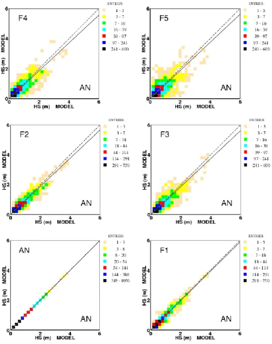
The results reported in the previous section concern the anal-ysis data. We now move to the corresponding forecasts. At this aim we intercompare the analysis wave heights with the corresponding data forecast one day before (0–24 h), two days before (24–48), and so on till the forecast issued five days before. The comparison is done at the tower and at the three considered buoys (see Fig. 3). Clearly, in relation to the conditions in front of the Venice lagoon, the tower is the main point of interest.
The full comparison for the tower is given in Fig. 12, where F1, F2, F3, F4, F5 represent, respectively, the one, two,. . . , five day forecasts. Taking the analysis as reference condition, we see little difference with the forecast fields. There is a tendency toward a mild underestimate, always less than 7 %, of the significant wave height going toward the longest forecast range. We see the expected increase of scat-ter index, the overall indicating that the forecast is correct on average, with an uncertainty on the exact “where and when” for forecasts well ahead in time. However, it is worthwhile to point out that up to day three, the scatter index is lower than the one out of the intercomparison between model and altimeter data. This is a strong indication of the reliability of the forecasts with respect to the analysis.
The intercomparison with the tower and buoy data is sum-marised in Table 4, respectively, for the one, two, .., five day forecasts. The conclusions about the buoys are similar to the ones done for the tower. Basically, the forecasts are always consistent with the corresponding analysis. The scatter in-dices increase with the range of the forecast. We will discuss this issue in more detail in the final section.
Table 4.Statistics for the comparison between the forecasts of the significant wave heights at different range (one to five days) and the corresponding analysis. The locations considered are the ISMAR oceanographic tower and the three wave recording buoys. See Fig. 3 for their positions. The considered period is 2010.
day 1 tower Ancona Pescara Monopoli
mean 0.52 0.72 0.82 0.67 best-fit slope 1.00 0.94 0.99 1.18 bias 0.01 −0.04 −0.04 0.11 scatter index 0.21 0.35 0.34 0.42
day 2 tower Ancona Pescara Monopoli
mean 0.52 0.72 0.82 0.67 best-fit slope 0.95 0.92 0.93 1.20 bias −0.01 −0.06 −0.08 0.12 scatter index 0.43 0.38 0.34 0.47
day 3 tower Ancona Pescara Monopoli
mean 0.52 0.72 0.82 0.67 best-fit slope 0.96 0.89 0.92 1.22 bias −0.01 −0.08 −0.08 −0.12 scatter index 0.47 0.42 0.39 0.52
day 4 tower Ancona Pescara Monopoli
mean 0.52 0.72 0.82 0.67 best-fit slope 0.95 0.88 0.92 1.20 bias −0.01 −0.08 −0.05 0.12 scatter index 0.52 0.46 0.45 0.56
day 5 tower Ancona Pescara Monopoli
mean 0.52 0.72 0.82 0.67 best-fit slope 0.93 0.92 1.04 1.21 bias −0.02 −0.06 0.00 0.11 scatter index 0.55 0.54 0.55 0.58
8 The use of wave information for tidal forecast
Having described in general, but quantitatively, terms of the performance of the wave forecast system in the Adriatic Sea, and in particular in its northern section, we now concentrate on the use of this information for the forecast of the tidal level along the northern coasts of the basin, and in particular in the Venice lagoon. Figure 5 provides a good view of the north-ern Adriatic and, together with Fig. 3, of the position of the Venice lagoon on the upper-left side of the basin. Note (see also Fig. 4 for the overall reference) that the lagoon coastline is directly exposed to south-east, hence to the possible large waves associated to the sirocco storms. In this respect the Grado lagoon, shown at the upper end in the maps of Fig. 5, is shielded by the Istria peninsula, to the right in the figures.
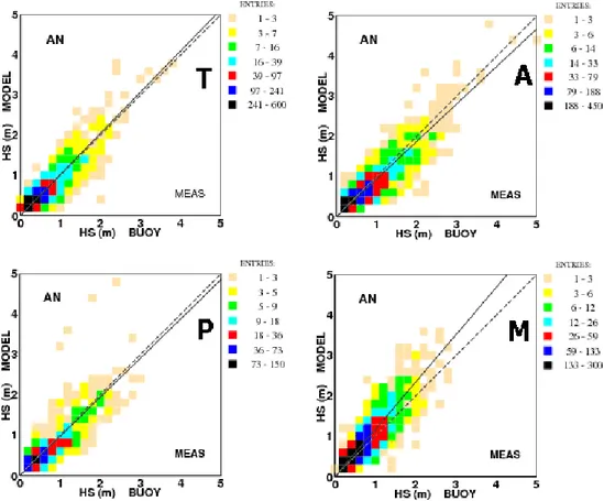
Fig. 9.Scatter diagrams of the model significant wave heights (analysis) vs the corresponding measured data at the ISMAR oceanographic tower (T) and the (A=Ancona), (P=Pescara), (M=Monopoli) wave measuring buoys. The period considered is 2006.
Chioggia, at about ten kilometre intervals. A closer view of the Lido inlet is given in Fig. 13. Each inlet is bordered by two jetties that protrude into the sea for quite a distance, about two kilometres in the case of Lido in Fig. 13. It is therefore evident that for the water level in the lagoon, the forcing factor is the tidal level at the end of the jetties.
The ICPSM has been producing tidal forecasts in the northern Adriatic, and in particular at Venice, since its foun-dation in 1981. When it stepped in with its operational hy-drodynamic models, it benefited from theoretical studies (see e.g. Tomasin and Frassetto, 1979) developed at the Vene-tian Laboratorio per lo Studio della Dinamica delle Grandi Masse, now part of ISMAR. At the beginning only statisti-cal models were used. They were progressively improved in time, from the simplest versions that only relied on the time series of the past, to the newest ones that take into account the predicted meteorological parameters (typically ECMWF pressure) and are “expert systems” capable of selecting a suitable set of coefficients, depending on the meteorologi-cal conditions. After 2002, hydrodynamic models were also operationally implemented at ICPSM, in particular a finite el-ement model of the Mediterranean Sea, the SHYFEM model developed at ISMAR-CNR of Venice (Bajo et al., 2007), and a finite difference model of the Adriatic Sea, the HYPSE
model developed at the University of Padua (Lionello et al., 2006). Both hydrodynamic models are forced by ECMWF pressure and wind fields.
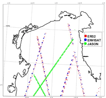
Fig. 10.Ground traces along which altimeter data is available in the northern Adriatic. The ERS-2 and ENVISAT satellites fly along the same orbit with a 30 day return period. Jason shows also the orbit of Topex and Jason-2, with a ten day return period.
Fig. 11.As Fig. 9, but for the northern Adriatic Sea (see Fig. 10). The total number of data is 3.927.
On 22 December 1979, a very severe sirocco storm hit the Adriatic, and in particular its northern part (see Cavaleri et al., 2010, for the hindcast of the storm). The associated flood ranks as the second highest in the Venice cronicles, soon be-hind the historical 1966 case. The storm was heavy enough to cause very severe damage to the superstructures of the IS-MAR oceanographic tower (see Fig. 2) located 15 km off-shore at a depth of 16 m just in front of the Lido and Malam-occo inlets. No wave record is available because the storm destroyed, among many other things, the batteries and the
re-lated cabling providing energy to the local wave recording system. Within the onboard mess two instruments survived, both mechanical: an anemometer that helped to make a faith-ful a posteriori evaluation of the storm, and a tide gauge, whose survival would deserve a longer description. In any case, in the aftermath of the storm we had available two tidal time series, one at the tower and another at the end of one of the jetties bordering the lagoon inlets. To our surprise, while the two gauges showed exactly the same tide history before and after the storm, there was an up to 40 cm difference be-tween the two time series during the storm, the higher values being at the coast. Given the conditions present during the storm, clearly exemplified in Fig. 14, we were inclined to as-sume a poor functioning of the tower gauge. The truth, as we soon learned, was different. When waves approach the coast and move into shallower water (see, among others, Holthui-jsen, 2007, for a discussion on the subject), after an initial set-down the bottom induced breaking leads to a loss of mo-mentum flux associated to the wave motion. This implies a gradual increase in the local water level from the seaward border of the surf zone towards the coast. The set-up, as it was defined by Bowen et al. (1968) and with the theory fully provided by Longuet-Higgins and Stewart (1964), may lead to remarkable differences between the offshore sea level and the one present at the coast. Bertotti and Cavaleri (1985) soon developed a model for its correct evaluation, and what at the beginning seemed a wrong record turned out to be an almost unique piece of information. Figure 15 shows clearly the relationship between the wave conditions estimated at the tower and the tidal difference with respect to the inlet pier tide-gauge. For our present purposes it is important to no-tice how taking this difference into account led to a good fit between the model and measured tidal levels at the coast.
Granted that this physical process was not considered in the hydrodynamic models, the question is why it was not naturally implicit in the tidal models mentioned above. Af-ter all, because, when implied by the conditions, the set-up is a permanent physical process, it should be automatically considered when fitting long time series of model and mea-sured data. The explanation comes with the presence of the jetties. We have pointed out that the tidal level acting as forc-ing for what happens within the lagoon is the one at the outer end of the jetties. However, the jetties protrude one or two kilometres into the sea, ending in relatively deep water. Six metre is the depth of the undisturbed isobath at the level of their outer end. A rule-of-thumb estimate (see Bowen et al. 1968, and Holthuijsen, 2007) suggests about 2.5 m as maxi-mum possible significant wave height at this depth (40 % of the local depth). Therefore, the set-up will be present at this level, hence in the lagoon, only when the waves are above this height, hence subjected to bottom induced breaking at this distance from the coast. For lowerHsvalues, set-up will
Fig. 12. Scatter diagrams between the significant wave heights out of the model F1 = one, F2 = two, F3 = three, F4 = four, F5 = five day forecasts and the corresponding analysis (AN). The considered period is 2010.
inlets). In this case a set-up is still present at the coast, of course lower than in the worst storms, and irrelevant for the tidal level in the lagoon. Note that the specific behaviour of the waves in the tidal channels depends on the phase, flow or ebb, of the tide.
We have previously mentioned that the statistical and nu-merical models have been formulated to fit the historically recorded tidal data. For what was just said, this implies a fit with the data recorded at the tide gauges at the jetty outer ends (or within the lagoons – for the present purposes the problem is the same). However, the set-up is here a rare event, only associated to the worst storms. Besides, in our
Fig. 13. The Lido inlet to the Venice lagoon. The length of the jetties is about 2 km.
Fig. 14.The tidal record of 22 December 1979 at the tower (thick line – see Fig. 2) and at the end of one of the jetties bordering the inlets to the lagoon (see Fig. 13). The horizontal spacing is one hour, the vertical one 10 cm (after Cavaleri, 1999).
15 km offshore. A rule-of-thumb estimate (coastal set-up≈ 1/6 of offshoreHs) suggests that up to one metre set-up was
present all along the northern coast of the Adriatic.
Although present, as just mentioned, in 0.1 % of the cases (order of magnitude), it is clearly important to consider wave set-up in the hydrodynamic tidal forecast of the worst cases. ICPSM is presently considering implementing it in its oper-ational models. On the other hand, it sounds difficult to take
Fig. 15. (a)recorded water level and astronomical tide at Venice during the 22 December 1979 event.(b)recorded storm surge level (difference of the graphs in (a)and model prediction. (c) wave height at the tower, evaluated and recorded wave set-up at the har-bour entrance.(d)recorded storm surge level (same as(b)) and cor-responding surge+set-up model results (after Cavaleri et al., 1991).
it into consideration in the statistical models simply because, as already discussed, it is a rare event, at least at the harbour entrances whose level controls the one in the lagoon. In prin-ciple, given the wave model results, one should isolate the cases when set-up is present at the harbour entrances and de-rive specific statistical relationships for these cases. Know-ing the correspondKnow-ing tidal level to use the correct bottom depths, another possible approach is to derive the set-up from the wave model and add it to the tidal results. This would im-ply a second order error with respect to the already evaluated set-up because the used depths would not consider the added set-up. Apart from the possibility of an iteration, the associ-ated error would only be of second order magnitude. Work along these lines is in progress.
9 Discussion and conclusions
activities and for the purposes of ICPSM. This confirms what we said at the beginning of this paper, i.e. that the ECMWF wind over the Adriatic is basically correct, at least as gen-eral structure of the fields, but characterised by too low wind speeds. It follows that for every specific resolution of the input fields, a simple but carefully chosen objective correc-tion, derived once forever from extensive comparisons of both wind and wave data with satellite and buoy measured quantities, is capable of producing wind data that, although not of the same quality as the ones available for the oceans, lead to quite satisfactory results for all practical purposes. Clearly, this does not exclude that it may be possible to reach further improvements. For this purpose we now focus on the limited but present errors recognised in the wave model results, discussing their possible genesis and the related im-provements.
When comparing model vs ENVISAT altimeter data on the whole basin, we had called attention to some character-istics of the results, namely: (a) a level of performance that, although at a limited level, seems to vary from year to year (see Table 1), (b) an overestimate of the higher wave heights (see Fig. 8), (c) a larger overestimate when moving towards the southern part of the basin, and (d) a mild underestimate in the northern part. All these features can be related with the interaction of the meteorological fields with the orography that surrounds the Adriatic. This interaction implies substan-tial modifications in the local fields that are only partly well reproduced in the results of the meteorological model.
We quoted the correct geometry of the ECMWF fields, with an underestimate of the surface wind velocity above the sea. The reason of this underestimate is related (see Cava-leri and Bertotti, 2004) to a limited reactivity of the model surface boundary layer when the wind passes from land to sea. As an order of magnitude, in the sea this implies dou-bling the wind speed within 50 km from the coast. In the ECMWF model this change happens more slowly, reaching a regime situation after 200 km or more, a distance that de-creases when the model resolution inde-creases (it is fair to men-tion that some progress in this respect has been done in the most recent period). This implies a rather large coastal zone where the wind is underestimated. While this happens also on the ocean coastal zones, for the overall statistics of the model performance this fact is clearly irrelevant when com-pared to the large dimensions of the basin. However, when the dimensions of the basin decrease, as is the case in the Mediterranean and more so in the Adriatic where the area of underestimate is similar to the dimensions of the basin, then U10 appears underestimated in the whole basin of
in-terest. This is clearly the case in the Adriatic. However, it is also clear that the fetch, i.e. the distance run by wind on the sea, depends on the location and the wind direction. Given the shape of the Adriatic (see Fig. 3), bora has a lim-ited fetch and it is therefore more underestimated than the sirocco that, blowing along the main axis of the basin, has a fetch up to 700 km. It follows that the use of a single
cor-rection coefficient, unavoidably mediated between the two situations, leads to an underestimate of the bora wind, hence wave heights, and an overestimate of the sirocco ones.
The yearly variations of the performance of the model seen in Table 1 corresponds to the different dominating climatolo-gies in the single years. The different position of the Azores anticyclone, e.g. more to the east or to the west, implies that the Atlantic storms enter the Mediterranean respectively more from the north or from south-west. In a very simplified manner these two situations correspond to the dominance of bora or sirocco in the Adriatic Sea.
Although bora is, as a rule, the strongest wind, it is sirocco that, thanks to the extended fetch, leads to the largest wave heights in this basin. It follows that we overestimate the largestHsvalues, exactly what we have seen in Fig. 8.
Be-sides, bora does not in general affect the southern part of the Adriatic, where the maximum wave heights are due to north-west winds. Therefore, in this area we can expect, as it is indeed the case, an overestimate of the model results.
It is clear that the specific solution for a given basin, in our case the Adriatic, is the use of different coefficients accord-ing to area and wind direction. This approach has already been followed and it has indeed led to some improvement. The practical problem is how frequently these coefficients need to be updated following the progressive changes and in-creased resolution of the ECMWF meteorological model. As we already mentioned, increasing the resolution leads in gen-eral to an improvement of the surface wind fields, hence to a variation of the related coefficients. Besides the improved orographic description, it leads to a better spatial descrip-tion of the bora within the narrow valleys of the Dinaric Alps through which the wind preferentially blows before jettying out into the sea. The point is that it is relatively simple to establish a single coefficient using, for instance, one year of model data, in so doing reaching a reliable result. However, the volume of data required for a similar determination of several coefficients (e.g. the north, central and south parts of the basin plus four or more directional sectors) increases proportionally to the number of coefficients. This is diffi-cult because the model is updated relatively frequently. In practice, by the time we have enough data at our disposal, most likely the model will be moved to the next cycle or res-olution. Presently, following the implementation of the high resolution T1279 version of the meteorological model, we are working to see if it is possible to reach a compromise solution within a relatively short time.
since July 2008, and therefore it cannot be used to derive the long time series required for a reliable estimate of the climate that characterises the Mediterranean – time series required to derive, among other things, a possible climate trend. On the contrary, Henetus has been operational since 1996 with prac-tically constant characteristics of its results, therefore provid-ing, although within 14 yr, reliable statistics. Note that, while in principle it would be possible to use the present systems, e.g. NETTUNO, to hindcast the past conditions, the human and computer efforts required, mainly for the meteorologi-cal model, is such to make such action practimeteorologi-cally impossible should we use the present resolution. As a matter of fact similar actions exist and have been done (see, among oth-ers, Lionello and Galati, 2008). However, for the mentioned reasons the resolution used for these projects is much lower than the present ones. In what is probably the most exten-sive effort in this respect, ECMWF (see Uppala et al., 2005) used a T159 resolution, corresponding to about 125 km, for its extensive reanalysis covering the period 1957–2002. Al-though then corrected with downscaling, the approximations involved in areas characterised by strong spatial gradients, and in particular in the smaller basins, make the related re-sults less reliable in these specific areas.
As forecast the Henetus results are very good, at least till day 4, and fully consistent with the analysis ones. Given that the wave model results are fully dependent on the quality of the driving wind fields, we can derive also the high quality of the ECMWF meteorological forecasts. The closeness to uni-tary slope of the best-fit lines seen in Table 4 strongly sug-gests that the ECMWF model retains also in the forecasts, till five days in our case, the dynamical characteristics that lead, using data assimilation, to the analysis. As a matter of fact, at least within the forecast range considered in the Adri-atic, in general the error of a forecast is not in ‘what’ but in ‘where’ and ‘when’. The determinism of the model provides the specific time and location of a given event. The practical problem is which is the sensitivity of the wave results to a small shift, in time and space, of the meteorological input. In a small basin such as the Adriatic, minor forecast errors, for instance about the position of a cold front, may have dras-tic consequences. A classical example, although concerning mainly tidal forecast, is given by Cavaleri et al. (2010). The shown coherence between wave analysis and forecast data clearly shows that these meteorological errors are indeed lim-ited. However, the events affecting the Adriatic are often short, and even a small time or space error of the driving wind fields may lead to some differences between analysis and forecast of the situation at a given time. The implications for the statistics shown in Table 4 are not in the slope of the best-fit lines (the climatologies remain consistent), but in the increase of the scatter index SI, i.e in a wider distribution of the points around the best-fit lines. Note, however, that this increase concerns more the low values of wave height. This should be expected, because the cited time and space errors are likely to be more frequent and relatively larger for
situa-tions not characterised by a large-scale, well-defined meteo-rological structure. Wherever everything depends on a small detail of the field, the variability, especially the forecast one, is larger.
The results of Henetus are fully available to the pub-lic, who can explore the full results at the two web-sites www.comune.venezia.it/maree, in the section dedicated to the forecasts, and www.ismar.cnr.it.
Acknowledgements. We are pleased to acknowledge the helpful
and constructive comments by the two reviewers.
Edited by: A. Mugnai
Reviewed by: M. Gomez and T. Soomere
References
Bajo, M. and Umgiesser, G.: Storm surge forecast through a com-bination of dynamic and neural network models, Ocean Model., 33, 1–9, doi:10.1016/j.ocemod.2009.12.007, 2010.
Bajo, M., Zampato, L., Umgiesser, G., Cucco, A., and Canestrelli, P.: A finite element operational model for the storm surge prediction in Venice, Estuar. Coast. Shelf S., 75, 236–249, doi:10.1016/j.ecss.2007.02.025, 2007.
Bertotti, L. and Cavaleri, L.: Coastal set-up and wave breaking, Oceanol. Acta, 8, 2, 237–242, 1985.
Bertotti, L., Cavaleri, L., De Simone, C., Torrisi, L., and Vocino, A.: Il sistema di previsione del mare “NETTUNO”, Riv. Meteorol. Aeronautica, 25–36, January–March 2010.
Bidlot, J.-R., Holmes, D. H., Wittmann, P. A., Lalbeharry, R., and Chen, H. S.: Intercomparison of the performance of operation ocean wave forecasting systems with buoy data, Weather Fore-cast., 17, 287–310, 2002.
Bonavita, M. and Torrisi, L.: Impact Of a Variational Objective Analysis Scheme On a Regional Area Numerical Model: The Italian Air Force Weather Service Experience, Meteorol. Atmos. Phys., 88, 1–2, 2005.
Bowen, A. J.,Inman, D. L., and Simmons, V. P.: Wave “set-down” and “set-up”, J. Geophys. Res., 73, 8, 2569–2577, 1968. Canestrelli, P. and Moretti, F.: I modelli statistici del Comune di
Venezia per la previsione della marea: valutazioni e confronti sul quinquennio 1997–2001, Atti dell’Istituto Veneto di Scienze Lettere ed Arti, Tomo CLXII, 479–516, 2004.
Canestrelli, P. and Zampato, L.: Sea level forecasting at the Cen-tro Previsioni e Segnalazioni Maree of the Venice Municipality, in: Flooding and Environmental Challenges for Venice and its Lagoon: State of Knowledge, edited by: Fletcher, C. A. and Spencer, T., Cambridge University Press, 85–97, 2005.
Canestrelli, P. and Tosoni, A.: L’evoluzione dei modelli stocastici a Venezia: una nuova struttura previsionale di tipo esperto, sub-mitted, 2011.
Cavaleri, L.: The oceanographic tower Acqua Alta – activity and prediction of sea states at Venice, Coast. Eng., 39, 29–70, 2000. Cavaleri, L., Bertotti, L., and Lionello, P.: Extreme storms in the
Adriatic Sea, in: Proceedings 22nd Int. Conf. on Coastal Eng., edited by: Edge, B. L., 218—226, Delft, The Netherlands, 2–6 July 1990, Publ. ASCE, 3, 305, 1991.
Cavaleri, L. and Bertotti, L.: Accuracy of the modelled wind and wave fields in enclosed seas, Tellus, 56A, 167–175, 2004. Cavaleri, L. and Bertotti, L., The improvement of modelled wind
and wave fields with increasing resolution, Ocean Eng., 33, 5–6, 553–565, 2006.
Cavaleri, L., Bertotti, L., Buizza, R., Buzzi, A., Masato, V., Umgiesser, G., and Zampato, M.: Predictability of extreme meteo-oceanographic events in the Adriatic Sea, Q. J. R. Meteor. Soc., 400–413, doi:10.1002/qj.567, February 2010.
De Boni, M., Cavaleri, L., and Rusconi, A.: The Italian waves mea-surement network, Proc. 23rd Int. Conf. on Coastal Eng., 1840– 1850, Venice, 3516, 4–9 October 1992, 1993.
Holthuijsen, L. H.: Waves in Oceanic and Coastal Waters, Cam-bridge University Press, 397 pp., 2007.
Janssen, P. A. E. M.: Progress in ocean wave forecasting, J. Com-put. Sci., 227, 7, 3572–3594, 2008.
Janssen, P. A. E. M., Bidlot, J.-R., Abdalla, S., and Hersbach, H.: Progress in ocean wave forecasting at ECMWF, Tech. Memo. 478. ECMWF, 27 pp., 2005.
Komen, G. J., Cavaleri, L., Donelan, M., Hasselmann, K., Hassel-mann, S., and Janssen, P. A. E. M.:Dynamics and Modelling of Ocean Waves, Cambridge University Press, 532 pp., 1994. Lionello, P.: Mediterranean wave climate variability and its links
with NAO and Indian monsoon, Clim. Dynam., 25, 611–623, 2005.
Lionello, P., Sanna, A.,Elvini, E., and Mufato, R.: A data assimi-lation procedure for operational prediction of storm surge in the northern Adriatic Sea, Cont. Shelf Res., 26, 539–553, 2006. Lionello, P. and Galati, M. B.: Links of the significant wave height
distribution in the Mediterranean sea with the Northern Hemi-sphere teleconnection patterns, Ad. Geosci., 17, 13–18, 2008. Longuet-Higgins, M. S. and Stewart, R. W.: Radiation stresses in
water waves: a physical discussion with applications, Deep-Sea Res. Pt., 11, 529–562, 1964.
Palmer, T. N., Buizza, R., Leutbecher, M., Hagedorn, R., Jung, T., Rodwell, M., Virat, F., Berner, J., Hagel, E., Lawrence, A., Pappenberger, F., Park, Y.-Y., van Bremen, L., Gilmour, I., and Smith, L.: The ECMWF Ensemble Prediction System: recent and on-going developments. A paper presented at the 36th Ses-sion of the ECMWF Scientific Advisory Committee. ECMWF Research Department Technical Memorandum n. 540, ECMWF, Shinfield Park, Reading RG2-9AX, UK, 2007.
Richardson, D. S., Bidlot, J., Ferranti, L., Ghelli, A., Gibert, C., Hewson, T., Janousek, M., Prates, F., and Vitart, F.: Verifica-tion statistics and evaluaVerifica-tions of ECMWF forecasts in 2008– 2009, ECMWF Tech. Memo. 606. ECMWF, Reading, U.K., 47 pp., available at http://www.ecmwf.int/publications/library/ do/references/list/14, 2010.
Simmons, A.: Observation, assimilation and the improvement of global weather prediction – some results from operational fore-casting and ERA-40, in: Predictability of Weather and Climate, Cambridge University Press, 428–528, 2006.
Simmons, A. and Hollingsworth, A.: Some aspects of the improve-ment in skill of numerical weather prediction, Q. J. Roy. Meteor. Soc., 128, 647–677, 2002.
Simmons, A., Mureau, R., and Petroliagis, T.: Error growth and predictability estimates for the ECMWF forecasting system, Q. J. Roy. Meteor. Soc., 121, 1739–1771, 1995.
The WISE Group – Cavaleri, L., Alves, J.-H. G. M., Ardhuin, F., Babanin, A., Banner, M., Belibassakis, K., Benoit, M., Donelan, M., Groeneweg, J., Herbers, T. H. C., Hwang, P., Janssen, P. A. E. M., Lavrenov, I. V., Magne, R., Monbaliu, J., Onorato, M., Polnikov, V., Resio, D., Rogers, W. E., Sheremet, A., Smith, J. M. K., Tolman, H. L., van Vledder, G., Wolf, J., and Young, I.: Wave modelling – the state of the art, Prog. Oceanogr., 75, 4, 603–674, 2007.
Tomasin, A. and Frassetto, R.: Cyclogenesis and forecast of dra-matic water elevations in Venice, Mar. Forecast., edited by: Ni-houl, J. C. J., Elsevier, 427–437, 1979.
Uppala, S. M., Kallberg, P. W., Simmons, A. J., Andrae, U., da Costa Bechtold, V., Fiorino, M., Gibson, J. K., Haseler, J., Her-nandez, A., Kelly, G. A., Li, X., Onogi, K., Saarinen, S., Sokka, N., Allan, R. P., Andersson, E., Arpe, K., Balmaseda, M. A., Beljaars, A. C. M., van de Berg, L., Bidlot, J., Bormann, N., Caires, S., Chevallier, F., Dethof, A., Dragosavac, M., Fisher, M., Fuentes, M., Hagemann, S., Holm, E., Hoskins, B. J., Isak-sen, L., JansIsak-sen, P. A. E. M., Jenne, R., McNally, A. P., Manfouf, J.-F., Morcrette, J.-J., Rayner, N. A., Saunders, R. W., Simon, P., Sterl, A., Trenberth, K. E., Untch, A., Vasiljevic, D., Viterbo, P., and Woollen, J.: The ERA-40 Reanalysis, Q. J. Roy. Meteorol. Soc., 131, 2961–3012, 2005.
Valentini, A., Delli Passeri, L., Paccagnella, T., Patruno, P., Mar-sigli, C., Cesari, D., Deserti, M., Chiggiato, J., and Tibaldi, S.: The sea state forecast system of ARPA-SIM, Bollettino di Ge-ofisica Teorica e Applicata, 48, 333–349, 2007.