www.atmos-chem-phys.net/9/7923/2009/ © Author(s) 2009. This work is distributed under the Creative Commons Attribution 3.0 License.
Chemistry
and Physics
Technical Note: Formal blind intercomparison of OH
measurements: results from the international campaign HOxComp
E. Schlosser1, T. Brauers1, H.-P. Dorn1, H. Fuchs1, R. H¨aseler1, A. Hofzumahaus1, F. Holland1, A. Wahner1, Y. Kanaya2, Y. Kajii3, K. Miyamoto3, S. Nishida3, K. Watanabe3, A. Yoshino3, D. Kubistin4, M. Martinez4, M. Rudolf4, H. Harder4, H. Berresheim5,*, T. Elste5, C. Plass-D ¨ulmer5, G. Stange5, and U. Schurath6 1Forschungszentrum J¨ulich, ICG-2: Troposph¨are, 52425 J¨ulich, Germany
2Frontier Research Center for Global Change (currently Research Institute for Global Change), Japan Agency for
Marine-Earth Science and Technology, Yokohama 236-0001, Japan
3Tokyo Metropolitan University, Department of Applied Chemistry, Tokyo 192-0397, Japan 4Max Planck Institute for Chemistry, Atmospheric Chemistry Dept., 55020 Mainz, Germany 5Deutscher Wetterdienst, Meteorol. Observatorium, 82383 Hohenpeissenberg, Germany 6Forschungszentrum Karlsruhe, IMK-AAF, 76021 Karlsruhe, Germany
*now at: National University of Ireland Galway, Department of Physics, Galway, Ireland
Received: 26 May 2009 – Published in Atmos. Chem. Phys. Discuss.: 26 June 2009 Revised: 16 September 2009 – Accepted: 23 September 2009 – Published: 22 October 2009
Abstract. Hydroxyl radicals (OH) are the major oxidiz-ing species in the troposphere. Because of their central importance, absolute measurements of their concentrations are needed to validate chemical mechanisms of atmospheric models. The extremely low and highly variable concentra-tions in the troposphere, however, make measurements of OH difficult. Three techniques are currently used worldwide for tropospheric observations of OH after about 30 years of technical developments: Differential Optical Laser Ab-sorption Spectroscopy (DOAS), Laser-Induced Fluorescence Spectroscopy (LIF), and Chemical Ionisation Mass Spec-trometry (CIMS). Even though many measurement cam-paigns with OH data were published, the question of accu-racy and precision is still under discussion.
Here, we report results of the first formal, blind in-tercomparison of these techniques. Six OH instruments (4 LIF, 1 CIMS, 1 DOAS) participated successfully in the ground-based, international HOxComp campaign carried out in J¨ulich, Germany, in summer 2005. Comparisons were per-formed for three days in ambient air (3 LIF, 1 CIMS) and for six days in the atmosphere simulation chamber SAPHIR (3 LIF, 1 DOAS). All instruments were found to measure tro-pospheric OH concentrations with high sensitivity and good time resolution. The pairwise correlations between differ-ent data sets were linear and yielded high correlation coef-ficients (r2=0.75−0.96). Excellent absolute agreement was
Correspondence to:H.-P. Dorn ([email protected])
observed for the instruments at the SAPHIR chamber, yield-ing slopes between 1.01 and 1.13 in the linear regressions. In ambient air, the slopes deviated from unity by factors of 1.06 to 1.69, which can partly be explained by the stated instru-mental accuracies. In addition, sampling inhomogeneities and calibration problems have apparently contributed to the discrepancies. The absolute intercepts of the linear regres-sions did not exceed 0.6×106cm−3, mostly being
insignif-icant and of minor importance for daytime observations of OH. No relevant interferences with respect to ozone, water vapour, NOx and peroxy radicals could be detected. The
HOxComp campaign has demonstrated that OH can be mea-sured reasonably well by current instruments, but also that there is still room for improvement of calibrations.
1 Introduction
excited oxygen atoms with water vapour.
O3+hν→O(1D)+O2 (R1)
O(1D)+H2O→2 OH (R2)
Minor sources are the photolysis of nitrous acid (HONO) and hydrogen peroxide, and the ozonolysis of alkenes. The ma-jor secondary OH source, i.e. from other radical species, is the reaction of nitric oxide (NO) with hydroperoxy radicals (HO2). Lifetimes of OH vary between 1 s and 10 ms in clean
and polluted environments, respectively, due to the rapid reactions of OH with atmospheric trace gases. Given the high reactivity and correspondingly short lifetime, the tro-pospheric OH concentration is generally low (sub-ppt) and highly variable. At night, when the photolytic production vanishes, OH concentrations have been observed at levels as low as a few 104cm−3in clean marine air (Tanner and Eisele,
1995), up to values around 106cm−3at a forest site (Faloona
et al., 2001). At daytime when OH generally correlates well with solar UV flux, concentrations can reach maximum val-ues of 107cm−3(0.4 ppt) at noon in clean and polluted envi-ronments (e.g. Hofzumahaus et al., 1996; Eisele et al., 1996; Martinez et al., 2008).
Since the 1970s OH radicals are recognised to be the ma-jor oxidant in the atmosphere converting more than 90% of the volatile organic matter (Levy, 1974). Since then many attempts were made to measure OH concentrations in the troposphere by various techniques (see review by Heard and Pilling, 2003). For the first time tropospheric OH was de-tected by Perner et al. (1976) in J¨ulich using Differential Optical Absorption Spectroscopy. DOAS based OH instru-ments were also developed in Frankfurt (Armerding et al., 1994) and Boulder (Mount et al., 1997). However, currently only one instrument is being operated by the J¨ulich group in field and chamber campaigns (Dorn et al., 1996; Brauers et al., 2001; Schlosser et al., 2007). The most widely applied OH measurement technique is Laser-Induced Fluorescence (LIF) combined with a gas expansion, also known as Fluo-rescence Assay with Gas Expansion (FAGE) (e.g. Hard et al., 1984; Stevens et al., 1994; Holland et al., 1995; Creasey et al., 1997; Kanaya et al., 2001; Dusanter et al., 2008; Mar-tinez et al., 2008). LIF instruments directly measure OH with high sensitivity and can be built compact for mobile operation. Chemical-Ionisation Mass-Spectrometry (CIMS) is an indirect OH measurement technique with very high sensitivity and good mobility for ground and aircraft field campaigns comparable to LIF instruments (Eisele and Tan-ner, 1991; Berresheim et al., 2000). Long term monitor-ing of OH concentrations has only been demonstrated us-ing CIMS (Rohrer and Berresheim, 2006). All three tech-niques (DOAS, LIF, CIMS) involve elaborate, expensive, custom-made experimental setups with vacuum pumps, laser systems, and/or mass spectrometers. Therefore, worldwide less than ten groups measure atmospheric OH using these techniques. Other techniques, e.g. the salicylic acid scav-enger method (Salmon et al., 2004) or the radiocarbon tracer
method (Campbell et al., 1986) do not reach the quality stan-dards of accuracy, sensitivity and time resolution provided by LIF, CIMS, and DOAS.
Atmospheric OH radicals have been elusive and hard to measure (Brune, 1992), because:
– low OH concentrations require extremely sensitive de-tection techniques, which are not readily available, – OH reacts efficiently at wall surfaces requiring
precau-tions to avoid instrumental OH loss,
– most other atmospheric species are much more abun-dant, raising the potential for interferences in OH detec-tion,
– stable calibration mixtures for OH do not exist; there-fore, calibration requires a technical OH source which produces accurately known amounts of OH radicals. Initial attempts to measure atmospheric OH by DOAS were successful, but required very long absorption path lengths (10 km) and long integration times of about 1 h (Perner et al., 1987; Platt et al., 1988). Attempts in the 1970s and 1980s to measure atmospheric OH by LIF and the radio-carbon tracer method failed as a result of insufficient detec-tion sensitivity, poor technical performance or interference problems. This was demonstrated in an OH intercomparison of two LIF instruments and one radiocarbon technique during the CITE 1 mission 1983/84 (Beck et al., 1987) and a corre-sponding NASA funded expert workshop on HxOy
measure-ments (Crosley and Hoell, 1986). The self-generation of OH by laser photolysis of ozone (reactions R1 and R2) turned out to be a major obstacle that hindered reliable OH measure-ment by LIF methods for many years (see Smith and Crosley, 1990, and references therein). In the beginning of the 1990s, major progress was achieved in terms of detection sensitiv-ities, development of calibration sources and suppression of interferences, providing the basis for fast, sensitive OH mea-surements by DOAS, LIF, radiocarbon tracer and the newly developed CIMS technique (Crosley, 1994). In the following years, given the experimental effort, only five intercompar-isons of atmospheric OH measurements were reported:
– A ground based OH photochemistry experiment (TOHPE) took place at Fritz Peak, Colorado, in 1991 and 1993. Four OH measurement instruments were de-ployed, but a meaningful intercomparison could only be done for two of them. The NOAA long path DOAS instrument (20.6 km path length using a retro-reflector) and the Georgia Tech CIMS instrument probed different parts of the atmosphere, but provided data with good correlation (r2=0.62) in 1993 (Mount et al., 1997). A linear fit to data (N=140) selected for clear days and low NOx revealed a slope (OH-CIMS/DOAS) of
– During a campaign at a clean-air-site near Pullman, in eastern Washington State, USA, in 1992, a LIF in-strument of the Portland State University (PSU) and a14CO radiocarbon instrument operated by Washing-ton State University (WSU) were involved (Campbell et al., 1995). The OH concentrations were near the limit of detection and the LIF instrument required an integra-tion time between 30 min and 60 min per measurement. The correlation coefficient for the two data sets was high (r2=0.74), but the slope of the regression was 3.9±1.01, indicating calibration problems.
– The J¨ulich DOAS (38.5 m between multi-path mirrors, 1.85 km total path length) and LIF instruments, both op-erated by the J¨ulich group, were compared during the field campaign POPCORN in rural Germany in 1994 (Brauers et al., 1996; Hofzumahaus et al., 1998). Ex-cluding a possibly contaminated wind sector, the instru-ments agreed well withr2=0.80 (N=137). The linear regression yielded a slope of 1.09±0.04 and an insignif-icant intercept.
– Two aircraft based campaigns were used to compare OH measurements of the NCAR CIMS instrument aboard the P-3B aircraft and those of the Penn State LIF in-strument aboard the NASA DC-8. During 1999 PEM Tropics B the ratio of the average OH measured by LIF/CIMS increased from 0.8 near the surface to 1.6 at 8 km altitude (Eisele et al., 2001). The TRACE-P cam-paign in 2001 involved three 0.5 h to 1.5 h comparison periods when the planes flew within 1 km distance. The correlation yielded ar2=0.88 and an approximate slope (CIMS/LIF) of 1.58 with a negligible intercept (Eisele et al., 2003). The OH data of the Penn State LIF were later revised because an error in the calibration of the primary standard, a photomultiplier tube (PMT) used to measure the photon flux, was found and the revised val-ues are a factor of 1.64 higher (Ren et al., 2008). A slope of 0.96 is found, i.e. the two instruments agree, if the slope reported earlier is divided by this factor.
– The J¨ulich DOAS (20 m between multi-path mirrors, 2.24 km total path length) and LIF instruments were again compared by the J¨ulich group in their atmo-sphere simulation chamber SAPHIR (Schlosser et al., 2007). The correlation was excellent (r2=0.93) based
on 400 data points. A marginal intercept and a slope of 0.99±0.13 were found.
In this study, we present the first formal, blind intercom-parison of OH measurements conducted as part of the Eu-ropean funded ACCENT program (Atmospheric Composi-tion of the Atmosphere: the European Network of Excel-lence). All international groups worldwide operating OH
in-1Reevaluated using a fit taking errors in both coordinates (Press and Teukolsky, 1992); 3.0±0.4 using standard regression.
struments were invited to participate. The groups from Ger-many (Deutscher Wetterdienst, Max-Planck Institut Mainz, Forschungszentrum J¨ulich), UK (University of Leeds) and Japan (Frontier Research Center for Global Change) took part in the corresponding campaign HOxComp (HOx
in-tercomparison) with seven different instruments (5 LIF-instruments, 1 CIMS, and 1 DOAS), each using their own calibration scheme. Due to an unfortunate laser system fail-ure, the instrument of the UK group (Creasey et al., 1997) did not produce any measurements. The following paper is therefore dealing with results of the remaining four groups (see Table 1). The campaign was performed as a two stage experiment with three days of measurements in ambient air and six days of measurements in the atmosphere simulation chamber SAPHIR on the campus of the Forschungszentrum in J¨ulich. The goal was the quality assurance of instruments used for detection of atmospheric OH (this work) and HO2
(Fuchs et al., 2009), addressing the following questions: – are current instruments (DOAS, LIF, CIMS) capable of
measuring atmospheric OH and HO2unambiguously? – are the measurements free of interferences?
– are the measurements correct and do they agree within the stated accuracies of their calibrations?
The whole process of formal blind intercomparison, the measurements and their evaluation, was independently refer-eed by Ulrich Schurath from Forschungszentrum Karlsruhe, Germany.
2 Experimental
2.1 The OH instruments
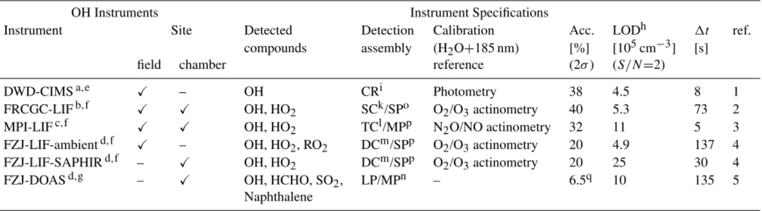
An overview and specifications of the six instruments that provided OH measurement data are given in Table 1. De-tailed descriptions are quoted in the last column, while sum-maries of the OH instruments are given in the following: 2.1.1 DOAS (FZJ), Forschungszentrum J ¨ulich,
Ger-many
Table 1.Instruments measuring OH during the HOxComp campaign.
OH Instruments Instrument Specifications
Instrument Site Detected Detection Calibration Acc. LODh 1t ref. compounds assembly (H2O+185 nm) [%] [105cm−3] [s]
field chamber reference (2σ) (S/N=2)
DWD-CIMSa,e X – OH CRi Photometry 38 4.5 8 1
FRCGC-LIFb,f X X OH, HO2 SCk/SPo O2/O3actinometry 40 5.3 73 2 MPI-LIFc,f X X OH, HO2 TCl/MPp N2O/NO actinometry 32 11 5 3 FZJ-LIF-ambientd,f X – OH, HO2, RO2 DCm/SPp O2/O3actinometry 20 4.9 137 4 FZJ-LIF-SAPHIRd,f – X OH, HO2 DCm/SPp O2/O3actinometry 20 25 30 4 FZJ-DOASd,g – X OH, HCHO, SO2, LP/MPn – 6.5q 10 135 5
Naphthalene
aDeutscher Wetterdienst, Hohenpeissenberg, Germany
bFrontier Research Center for Global Change, Yokohama, Japan cMax Planck Institute for Chemistry, Mainz, Germany
dForschungszentrum J¨ulich, J¨ulich, Germany eChemical Ionisation Mass Spectrometry fLaser Induced Fluorescence
gDifferential Optical Absorption Spectroscopy
hInstruments Limit of Detection (signal to noise ratioS/N
=2, while measuring blank at given time resolution) iChemical Reactor
kSingle Chamber lTandem Chamber
mDual Chamber (two separate inlets for OH and HO 2)
nSAPHIR Chamber, Long Path, Multi-Pass for Laser Absorption oSingle-Pass for Laser Excitation
pMulti-Pass for Laser Excitation
qmaximum uncertainty (Hausmann et al., 1997) References:
1: Berresheim et al. (2000)
2: Kanaya et al. (2001); Kanaya and Akimoto (2006) 3: Martinez et al. (2008)
4: Holland et al. (1995, 1998, 2003)
5: Dorn et al. (1995); Hausmann et al. (1997); Schlosser et al. (2007)
spectrum is de-convoluted by fitting a trigonometric back-ground and three to five reference spectra (OH, HCHO, a so far unidentified absorber X, and additionally SO2and
naph-thalene in case of ambient air measurements). The precision is calculated for each measurement from the bootstrap er-ror estimate and residual inspection by cyclic displacement (Hausmann et al., 1997, 1999). For this instrument the pre-cision was determined to be 1.2×106cm−3 for 135 s time intervals (Schlosser et al., 2007). Additional OH radicals may be formed by photolysis of O3 within the probe
vol-ume of the UV laser beam. The amount of this artificially produced OH depends, e.g. on the O3and H2O
concentra-tions, OH lifetime, the UV laser power, and the dwell time of the air within the volume probed by the laser beam (Dorn et al., 1995). Under adverse conditions that promote artifi-cial OH generation (high O3concentration (143 ppb), no air
movement in the dark chamber, long OH lifetime) an offset of (2.9±0.1)×106cm−3 per 1 mW of UV laser power was
detected (Schlosser et al., 2007). This effect was reduced by convection when the chamber was exposed to sunlight and when a fan was operated, e.g. during an experiment with high O3concentration which took place in the dark chamber on 22
July 2005. Additionally, the UV laser power was limited to maximum 1 mW and monitored to keep this interference well below 0.2×106cm−3.
2.1.2 LIF (FRCGC, FZJ, MPI)
Four LIF instruments contributed measurement data during this campaign (see Table 1). LIF can be used for the sen-sitive and fast direct detection of OH and the indirect de-tection of HO2 and RO2 after chemical conversion to OH.
Current techniques probe the OH radicals after expansion of ambient air through an inlet nozzle into a detection cham-ber at a pressure of a few hPa. Single rovibronic lines of the OH A26+(υ′=0)←X25(υ′′=0)transition are excited by pulsed UV laser light near 308 nm and resonance fluores-cence in the (307–311 nm) range is detected by gated photon counting perpendicular to the gas beam and the laser beam. The background signal, resulting from scattered laser radi-ation and solar stray light, is determined and subtracted for each OH measurement using an on- and off-resonance tun-ing cycle. Raw data is normalised ustun-ing the measured laser power and corrected for fluorescence quenching by water vapour. Calibration is performed with known concentrations of OH radicals, which are generated by photolysis of water vapour at 184.9 nm. The instruments vary in their technical details such as the nozzle and low pressure chamber geom-etry and volume, laser models and light guidance, detection volume geometry and detector types, architecture and cus-tom made calibration units (see below, Sect. A, and Table 1). All LIF instruments measured additionally HO2. The
mea-surement involves chemical conversion of HO2to OH by
ad-dition of NO in the gas expansion, followed by LIF detection of the additionally formed OH. The OH and HO2
measure-ments can be performed in a single chamber in an alternating mode or in two detection chambers, which are coupled or completely separated.
The FRCGC-LIF instrument of the Frontier Research Cen-ter for Global Change, Yokohama, Japan has been deployed in several field campaigns in Japan (Kanaya et al., 2007a,b). The setup includes a single detection cell, in which OH and HOxare measured alternately (Kanaya et al., 2001; Kanaya
and Akimoto, 2006). Short periods between these measure-ments are used to measure the background and to scan and to lock the laser wavelength. Concentrations of HO2are
calcu-lated from the difference of the measured HOxand 10
min-averaged OH levels. A black aluminum disk (halocarbon wax coated) was used as sun shade for ambient ments in order to reduce solar background in the measure-ment signals. In previous experimeasure-ments with a different laser system only a small power dependent correction for OH from the laser photolysis of ambient ozone has been established (Kanaya et al., 2007a). With the 10 kHz laser system used in the present work (average laser power: (5–9) mW at 308 nm) the correction is considered to be negligible.
Two LIF systems of the Forschungszentrum J¨ulich, Ger-many, were operated during the campaign. The FZJ-LIF-SAPHIR was used for measurements at the chamber only while the FZJ-LIF-ambient was used at the field site. Both
instruments differ in their setup, but are based on the same concept (Holland et al., 1995).
The FZJ-LIF-SAPHIR instrument was previously used for field campaigns (e.g. Hofzumahaus et al., 1996; Hol-land et al., 2003) and is now permanently installed at the SAPHIR chamber. FZJ-LIF-SAPHIR compared very well within 10% to FZJ-DOAS in previous tests (Hofzumahaus et al., 1998; Schlosser et al., 2007). For the present measure-ments, FZJ-LIF-SAPHIR was modified by replacing the for-merly used copper-vapour laser pumped dye laser system by a frequency doubled Nd-YAG (DPSS Spectra Physics Navi-gator I) pumped tuneable, frequency doubled dye laser (NLG Tintura) with a total laser power of (35–40) mW at 308 nm. The FZJ-LIF-SAPHIR instrument uses two detection cham-bers for separate detection of OH and HO2, each equipped
with its own inlet nozzle. The separation of the two detec-tion cells avoids potential contaminadetec-tion of the OH cell by NO which is used for HO2conversion in the other chamber.
In the current setup, ozone-related interference signals were not noted within the limit of OH detection for ozone concen-trations up to 260 ppbv at 1.4% of water vapour. Therefore, no ozone-related correction was performed in this work. The OH calibrations were reproducible from day to day within 5%, except for an unusually low OH detection sensitivity noted in the calibration of 22 July 2005. The measurements of this day were marked “not valid” to indicate a potential calibration problem. A large laser-power dependent back-ground signal led to a considerably higher OH detection limit of 25×105cm−3 (S/N=2, 1t=30 s) compared to earlier campaigns. The accuracy of the calibration is estimated to be 20% (2σ).
The FZJ-LIF-ambient instrument was first operated during the ECHO campaign (Kleffmann et al., 2005) using the same concept as FZJ-LIF-SAPHIR. The construction and operat-ing conditions of the OH and HO2detection chambers are
actually the same, but electronics, gas handling system and vacuum pump are designed to be smaller and light-weight, making the instrument suitable for mobile applications. The compact laser system (DPSS Photonics DS20-532; dye laser LAS Intradye) had a total UV power of 25 mW, which was directed sequentially through the OH and HO2 chambers,
and a reference cell for controlling the OH wavelength. An ozone interference of 0.7×104cm−3per ppb O3was
deter-mined and taken into account during evaluation. No power dependence for the parametrisation was needed, because the monitored laser power was virtually constant. The OH detec-tion limit was 5.3×105cm−3 (S/N
=2, 1t=137 s) and the reproducibility was 13%. The calibration and the accuracy is the same as for FZJ-LIF-SAPHIR.
The MPI-LIF instrument of the Max-Planck-Institut, Mainz, Germany was developed mainly for mobile platforms as a highly time resolved field instrument for OH and HO2
MPI-LIF design incorporates a Nd-YAG system as pump laser (2nd harmonic 532 nm, 2.6 W at 3 kHz) for an intra-cavity frequency doubled tunable dye laser. The wavelength is line-locked on the Q1(2) line signal from a reference cell in
which OH radicals are produced by H2O thermolysis using
a hot filament. Light is guided by UV-fibres to the detec-tion cells (average laser power coupled into the OH channel: (2–20) mW at 308 nm) and fluorescence is detected by mul-tichannel plates. Unlike the other LIF instruments it uses a multi-reflection cell (White system) to enhance the number of fluorescence photon counts and thus sensitivity and fea-tures a tandem detection cell setup. Ambient air is expanded through a nozzle into a low-pressure fluorescence cell where first OH radicals are detected by LIF. NO is then added to the gas beam that leaves the OH detection cell to convert HO2to
OH for the (indirect) HO2detection within the second
detec-tion cell. The cell geometries are designed to prevent a pol-lution of the OH detection cell with NO which is injected between OH and HO2stages, thereby preventing interference
of HO2with the detection of OH. In contrast to OH
measure-ments at daylight a significant and variable OH background signal was often observed at periods without daylight during experiments previous to HOxComp. Therefore all OH mea-surements by the MPI-LIF at times without daylight were submitted to the referee as not valid. The reason of this ef-fect is not yet understood. Studies have verified though that the interference is not due to laser-induced OH generation. 2.1.3 CIMS (DWD), Deutscher Wetterdienst,
Hohen-peissenberg, Germany
The DWD-CIMS instrument is usually installed at the Meteorological Observatory Hohenpeissenberg where it is in operation almost continuously since 1998 (see Rohrer and Berresheim, 2006). Its operation at the HOxComp field site was identical to the routine operation. The OH detection by CIMS is based on the work of Eisele and Tanner (1991) and has been described by Berresheim et al. (2000) with some modifications as outlined below.
The measurement principle includes continuous sampling of ambient air, followed by chemical titration, ion reaction, cluster dissociation, and mass selective detection. Ambient air (2400 slm) is pumped through a 100 mm wide tube with a smooth, ring shaped inlet. The central part of the flow is sampled 120 mm below the intake at a flow rate of 16 slm through a conical nozzle (10 mm diameter). 34SO2 is
in-jected at the front edge of the nozzle and forms H2SO4from
OH. Propane is added downstream to scavenge 98% of the recycled OH. The remaining 2% of recycled OH and am-bient H2SO4 are determined by background measurements
using propane instead of SO2 as OH scavenger. The
pro-cessed sample gas is transferred through a 900 mm long tube to the ion reaction zone where NO−3 ions are added to the sample from a sheath gas flow. H2SO4 is deprotonated by
NO−3 ions and then the ions are selectively transferred into
a vacuum system. Ion clusters are decomposed in a collision-dissociation unit and are refocused by electrical lenses to the quadrupole mass spectrometer (Extrel Inc.). An OH mea-surement cycle lasts 30 s, of which 8 s are used to obtain the ambient OH signal and another 8 s for the background signal. Modifications of the current instrument setup were applied since its description by Berresheim et al. (2000): (1) A noz-zle at the head of the sampling tube reduces disturbance in the titration zone due to cross-wind. (2) The sample inlet (nozzle) has been moved to 120 mm below the air inlet (from 300 mm) to minimise OH losses and chemical interferences in the inlet region. (3) The sample flow rate was increased from 10 slm to 16 slm yielding better signal-to-noise ratios and reduced chemical interferences in the titration zone. (4) The length of the sample tube transferring H2SO4 to the
ion reaction zone was changed from 300 mm to 900 mm (to transfer the gas through the ceiling of the laboratory at Ho-henpeissenberg). Losses in the nozzle and sample tube are routinely accounted for in calibration measurements.
The OH concentration is obtained after correction for background H2SO4and inlet chemistry, recycling OH from
NO+HO2, and OH-losses by CO, NMHC, and NO2. The
DWD-CIMS is designed for fairly clean atmospheric con-ditions, while in J¨ulich mostly polluted conditions were en-countered. Therefore, the correction factors to compensate for chemically induced changes of OH in the intake were higher than at Hohenpeissenberg, typically corrections of 30% with an uncertainty of ±11% were applied. An ac-curacy of 38% (2σ) results from the uncertainties of the CIMS calibration and the chemical correction factors dur-ing HOxComp. The precision of the OH measurements is 0.22×[OH]+0.19×106cm−3 (2σ, signal integration time: 8 s).
The CIMS instrument was operated during the ambient and chamber parts of the campaign. However, only the sam-ple tube with the nozzle was installed at SAPHIR, since in chamber experiments an intake flow of 2400 slm was not possible. Thus, the air intake system was substantially changed from routine operation and the use of the DWD-calibration-unit (Sects. 2.1.4 and A) was not possible. Al-though, for most times good and consistent results with other OH-measurement systems on a relative scale were achieved, it was decided to flag the results from the chamber as the sub-stantially modified intake-system had not been characterised and the sensitivity of the system could not be quantified ade-quately2.
2.1.4 Calibration
OH production is the photolysis of water vapour at 184.9 nm (mercury lamp) in a flow of (synthetic) air at ambient pres-sure, from which calibration gas is sampled (Aschmutat et al., 1994; Schultz et al., 1995; Kanaya et al., 2001; Bloss et al., 2004; Faloona et al., 2004; Martinez et al., 2008; Dusan-ter et al., 2008). The photolysis yields equal concentrations of OH and HO2,
H2O+hν →OH+H (R3)
H+O2+M→HO2+M (R4)
which can be calculated from a few experimental parameters:
[OH] = [HO2] =8σH2O[H2O]t (R5)
Here, σH2O is the well known absorption cross section
of water vapour at 184.9 nm. Its value of 7.14×10⁻²⁰cm2 (at 25◦C) measured by Cantrell et al. (1997) was confirmed within 2% by Hofzumahaus et al. (1997) and Creasey et al. (2000). The water vapour concentration[H2O]can be
mea-sured accurately, e.g. by a dew point hygrometer. The other parameters are the actinic flux8of the 184.9 nm radiation and the exposure timet of the calibration gas. Each experi-mental group (LIF, CIMS) had its own calibration device and its own method to measure8as explained in Appendix A. The resulting accuracies of the calibrations are listed in Ta-ble 1.
The DWD-CIMS instrument has a built-in calibration unit within the instrument’s main air inlet tube. OH radicals are produced during ambient air sampling from photolysis of at-mospheric water vapour by switching on a mercury lamp ev-ery 20 min for 5 min. In contrast, all LIF instruments have external radical sources, each of which consist of a flow tube, an illumination unit, and a supply of synthetic air. Calibra-tion measurements were usually performed once a day dur-ing the campaign. Measured OH calibration factors, which showed no significant variability or trend, were averaged for the following time periods: FRCGC-LIF (four periods): 10– 12, 17, 18, and 19–23 July 2005; FZJ-LIF-ambient: 10–12 July 2005, FZJ-LIF-SAPHIR: 17–23 July 2005 (excluding 22 July 2005); and MPI-LIF (two periods): 8–11 and 17–23 July 2005.
2.2 Measurement sites
The HOxComp campaign took place on the campus of the Forschungszentrum in J¨ulich (50◦54′33′′N, 06◦24′44′′E).
The instruments were set up within and partly on top of several containers. The formal part of the campaign in-cluded three days of ambient measurements from 9–11 July 2005 and six days of chamber experiments with the SAPHIR chamber from 17–23 July 2005. The weekend days 9–10 July 2005 had essentially no traffic on the campus of the Forschungszentrum.
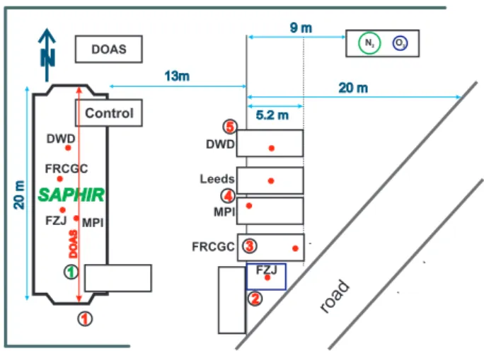
Fig. 1. Setup at the field site and at the SAPHIR chamber during HOxComp. Container placement east of SAPHIR with air sampling positions of the OH instruments marked as red dots. The DOAS light path is indicated in red within the chamber. Numbers indicate positions of supporting measurements: (1) NOx, O3, HCHO, VOC, H2O, CO; (2) temperature, relative humidity, HONO; (3) ultrasonic anemometer; (4) filter-radiometer; (5) O3. A road (closed for traf-fic) is located southeast and the site is bordered in the north and west by bushes and trees (marked by a green line). Liquid nitrogen and oxygen is stored in two tanks northeast of the chamber.
2.2.1 Field site
Ambient air measurements were located on the paved area between the institute building and the SAPHIR chamber (Fig. 1). The site is bordered by bushes, trees and a small road. The area is characterised by buildings, small roads, grassland and trees. The Forschungszentrum is surrounded by deciduous forest, agricultural areas, and main roads. The OH instruments were placed approximately 13 m east of the chamber side-by-side from north to south in the following or-der: DWD-CIMS, Leeds-LIF, MPI-LIF, FRCGC-LIF, FZJ-LIF-ambient with spacings between the instruments sam-pling inlets of approximately 2.9 m, 2.7 m, 3.2 m, and 4.5 m, respectively. All OH instruments sampled ambient air at about equal height (3.5 m) above ground. Standard instru-ments recorded humidity, NOx, O3, and meteorological data.
Additional measurements of HONO, hydrocarbons, and pho-tolysis frequencies were also conducted.
2.2.2 SAPHIR chamber
The atmosphere simulation chamber SAPHIR (Simulation of Atmospheric PHotochemistry In a Large Reaction Cham-ber) is designed to investigate tropospheric photochemistry under controlled chemical composition comparable to ambi-ent air at ambiambi-ent temperature, pressure and natural irradia-tion (e.g. Rohrer et al., 2005; Bohn and Zilken, 2005; We-gener et al., 2007; Poppe et al., 2007; Apel et al., 2008). It is constructed of a double-walled FEP cylinder (125 µm and 250 µm thickness; diameter 5 m, length 18 m, volume 270 m3), held by a steel frame and stabilised to 50 Pa above ambient pressure. In addition to the slight overpressure, the volume between inner and outer FEP film is flushed with clean N2to exclude contamination of the chamber by
ambi-ent air. The FEP foil has a 85% transmission for visible light, UV-A, and UV-B. A louvre-system allows fast shadowing of the chamber.
One chamber experiment was performed per day (17– 19, 21–23 July 2005). Each experiment started with overnight flushing of the dark chamber with ultra-pure synthetic air to reach low trace gas mixing ratios (NOx<10 ppt, CO<1 ppb, CH4<15 ppb, HCHO<50 ppt,
hydrocarbons<10 ppt, O3<1 ppb, and H2O<0.05 mbar). In
a second step Milli-Q water (Millipore) was evaporated and added to the purge flow to adjust the humidity. Trace com-pounds (e.g. O3, NOx, VOC, and/or CO) were then added
while mixing was assured by operation of a fan for 30 min. After complete gas mixing, intercomparison measurements were started. During the experiments, photochemistry was controlled by the louvre system which allowed the chamber to be exposed to or shielded from solar radiation. Periods of 1 h were scheduled for the addition of trace gases during the experiments. The louvre system was closed, followed by 30 min in the dark with no other changes. Then, the chem-ical composition was changed in the dark chamber with the fan turned on. Photochemistry was resumed by opening the louvre system.
The gas replenishment flow of (5–10) m3h−1of clean, dry synthetic air was used to compensate for sampling by ex-tractive measurements (4.5 m3h−1) and for leakage, which caused a dilution of (2–3)% h−1. Instruments were calibrated once a day subsequent to the experiments.
2.3 Data measurement protocol
The referee supervised all measurements and was the only person aware of all experimental details and authorised to change the experimental conditions. All groups synchro-nised their clocks (UTC, accuracy of time setting±1 s). Dur-ing the formal blind intercomparison measurements no com-munication of data or results was allowed between groups. Daily preliminary measurement data of each instrument was sent to the referee within 12 h after the end of an experiment. After the campaign, the groups prepared final data sets and questionable data was identified as part of the usual data anal-ysis by each group, but not removed. Instead it was marked
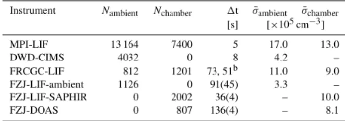
Table 2. Number of valid measurements (N), time interval (1t)a per measurement, and mean precision (σ¯) of the data measured dur-ing HOxComp.
Instrument Nambient Nchamber 1t σ¯ambient σ¯chamber [s] [×105cm−3]
MPI-LIF 13 164 7400 5 17.0 13.0
DWD-CIMS 4032 0 8 4.2 –
FRCGC-LIF 812 1201 73, 51b 11.0 9.0
FZJ-LIF-ambient 1126 0 91(45) 3.3 –
FZJ-LIF-SAPHIR 0 2002 36(4) – 10.0
FZJ-DOAS 0 807 136(4) – 8.1
aThe standard deviation (1σ) for the time interval is given in brack-ets if the acquisition time is irregular. If noσ is stated, fixed time intervals are listed.
bThe FRCGC-LIF changed the acquisition rate once.
“not valid” with a quality flag indicating the reason. In some cases data of whole days was marked “not valid” for indi-vidual instruments because uncertainties in the calibration were noted (e.g. 22 July 2005 of the FZJ-LIF-ambient and all 6 days of chamber measurements of the DWD-CIMS). The MPI-LIF marked all measurements in the dark “not valid” because of measurement artefacts. Final data was submit-ted to the referee eight weeks after the campaign. OH data was then disclosed and discussed among the HOxComp par-ticipants during a workshop in J¨ulich four months after the campaign.
The group operating the two FZJ-LIF instruments became aware of a systematic error within their calibration after the submission of their data to the referee. The reason was tech-nically simple but the error was not obvious and it had a sig-nificant effect on the calibration of the instrument. A mass flow controller which supplied synthetic air to the OH cali-bration unit had been incorrectly calibrated. This was discov-ered in 2006 during re-evaluation of a set of laboratory exper-iments that were performed before and after the HOxComp campaign in order to characterise the calibration unit. The revision entailed increases of the initially submitted OH con-centrations by factors of 1.26 and 1.28 for the FZJ-LIF-ambient and the FZJ-LIF-SAPHIR, respectively. An accor-dant revision of their submitted data was authorised by the referee after discussing the planned change with the other groups.
3 Results
3.1 Hydroxyl radical measurements
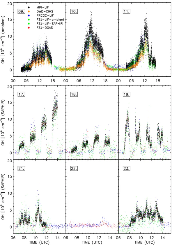
and at the SAPHIR chamber. The first row in Fig. 2 shows the data of the ambient measurements (MPI-LIF, DWD-CIMS, FRCGC-LIF, FZJ-LIF-ambient) and the lower two rows present all OH concentrations measured at the SAPHIR chamber (MPI-LIF, FRCGC-LIF, LIF-SAPHIR, FZJ-DOAS). Two instruments (MPI-LIF and FRCGC-LIF) sub-mitted valid data for both ambient and chamber experiments. On the 22nd, only the FRCGC-LIF and the FZJ-DOAS pro-vided valid data.
Ambient measurements include whole diurnal cycles dur-ing variable weather conditions, whereas chamber exper-iments were usually performed between 06:00 and 15:30 (UTC). There are no valid OH measurements of the MPI-LIF at night-time or when the louvre system of the chamber was closed as explained in Sect. 2.1. The number of submitted dataN and its mean precisionσ¯ observed during this cam-paign are listed for the instruments separately for ambient and chamber measurements in Table 2. The different mean measurement time intervals (1t) per OH measurement range from 5 s (MPI-LIF) to 136 s (FZJ-DOAS). Directly related to the different1t is the mean of precisions (σ¯), which ranged between 3.3×105cm−3(FZJ-LIF-ambient) to 17×105cm−3 (MPI-LIF) for this campaign’s data.
The MPI-LIF has the highest data acquisition rate (10 s) and thus collected the largest data set (Ntotal=20 564). Fast
measurements entail a lower precision, which is (17 and 13)×105cm−3for ambient and chamber measurements, re-spectively. The DWD-CIMS uses a similarly short integra-tion time of 8 s for each OH measurement, but the com-plete measurement cycle takes longer (30 s). No valid cham-ber measurements were submitted and Ntotal is thus only
4032. The average precision is 4.2×105cm−3. Like the
two previous instruments the FRCGC-LIF used a fixed time resolution, but it was changed during the campaign from 73 s to 51 s on 19 July. The mean precision was (11.0 and 9.0)×105cm−3. The FZJ-LIF-ambient used variable acqui-sition times (46 s to 355 s per measurement, mean 91 s). Time intervals were longer when the OH concentration was low in order to improve the limit of detection. The same ap-plies to the FZJ-LIF-SAPHIR (24 s to 74 s), but mostly1t was close to the mean of 36 s±4 s. Because of a high back-ground signal and noise of the fluorescence detector, but also because of the shorter acquisition time, the standard de-viation of the FZJ-LIF-SAPHIR data is 10×105cm−3, i.e. three times larger than the value for the FZJ-LIF-ambient (3.3×105cm−3). The FZJ-DOAS has the lowest average
time resolution with an almost fixed acquisition time of 136 s. The precision of the DOAS instrument depends on the opti-cal alignment and is independent of the OH concentration. The precision was on average 8.1×105cm−3.
3.2 Data processing
The original data of the participating instruments has very different time resolutions. Therefore, data sets for pairs of instruments were created using the original time intervals of the instrument with longer time intervals per measurement by processing the data of the instrument with the higher timer resolution: In case of multiple data points of the latter instru-ment within one time interval, the average and the standard deviation was calculated. These values reflect the statisti-cal and natural scattering of the OH measurements (external error) as well as the standard deviation stated for each mea-surement (internal error). This would be the preferred data basis for an intercomparison of two instruments, conserving the highest time resolution, because the natural OH concen-tration may vary rapidly according to the variable attenuation of sunlight. This variability is non statistical and not well rep-resented by the precision of the OH measurements leading to different weights in the analysis. However, for compar-ing several instruments, for improvcompar-ing the precision, and for representation a common time resolution is needed and de-termined by the instruments with the longest time intervals (FZJ-DOAS, FZJ-LIF-ambient). Data of all instruments was processed accordingly using 300 s time intervals that suit all participating instruments. Between pairs of instruments that are compared, the number of concurrent measurements is al-lowed to differ. The results of the analysis of the data aver-aged to the time intervals of the instrument with the lower time resolution were analysed as a check for consistency and confirm the findings presented in this paper.
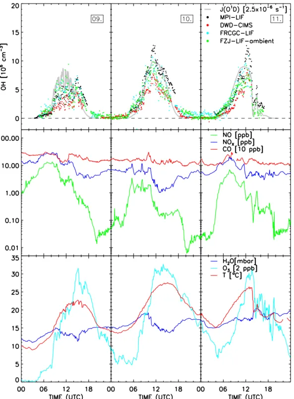
All valid OH measurements of the formal blind intercom-parison, converted to averages over common 300 s time in-tervals are shown in the first row of Figs. 3, 4, and 5. The two lower rows present important chemical and physical pa-rameters: NO and NOx, O3, CO, absolute humidity, and
tem-perature.
3.3 Ambient measurements
The ambient measurements covered a 3-day period (9–11 July 2005). The OH data of all instruments with some key parameters are shown in Fig. 3 (300 s average). The period was characterised by moderate temperatures for the season peaking at 28◦C on 10 July. While the first day started with
ground fog (until 08:10 UTC2) and was later characterised by scattered clouds (as seen from the strong fluctuations of the photolysis frequencies), the second day was almost cloud free. The sunny weather continued on the last day until 14:00, when a rain storm evolved. Wind came almost in-variably from northerly direction throughout all three days. Similar diurnal variations of trace gases were observed with high NOx in the morning hours (up to 30 ppb) and a
rela-tively constant CO of 200 ppb on average. Short CO peaks
up to 320 ppb were encountered on 10 July 2005 at 10:00 and the 11 July 2005 at 08:00. VOC concentrations were dom-inated by up to 1 ppb benzene and toluene, each. Isoprene concentrations reached 1.6 ppb in the evenings, but ranged between 0.3–0.6 ppb during daytime and below 0.3 ppb at night. Ozone showed a typical diurnal profile with very low mixing ratios at night and a strong increase starting at 06:00. Peak O3, however, was moderate and barely reached 70 ppb.
Not all OH instruments submitted valid data for the en-tire three day period, e.g. the MPI-LIF skipped night data for reasons discussed before and the FRCGC-LIF and the DWD-CIMS ceased measurements because of the weather conditions during the thunder storm of the last day. In ad-dition, no OH data was collected during times of calibration which were usually scheduled between 17:00 and 18:00, but the number and duration of calibration and maintenance pe-riods differed between the instruments.
The OH measurements by MPI-LIF, FRCGC-LIF, FJZ-LIF-ambient and DWD-CIMS show general good agree-ment, throughout all three days. The measured diurnal pro-files exhibit similar variations which are highly correlated to the ozone photolysis frequency, with maximum values at noontime and concentrations near zero at night. When looking in detail, differences between the instruments can be seen. For example, the peak values at noon differed signif-icantly between the instruments, most notably between the DWD-CIMS and the MPI-LIF that detected OH maxima of 8×106cm−3and 12×106cm−3, respectively. The FRCGC-LIF measured higher OH concentrations (0.7×106cm−3, 2σ/√N=0.1×106cm−3) during the night of 10 July 2005 to 11 July 2005 (21:00–03:00) compared to the other instru-ments (FZJ-LIF-ambient: (0.13±0.05)×106cm−3; DWD-CIMS: (0.09±0.02)×106cm−3). On the two last days, the LIF instruments of MPI and FZJ agree in the morning, but deviate (1–3)×106cm−3from each other after 10:00. 3.4 Chamber measurements at SAPHIR
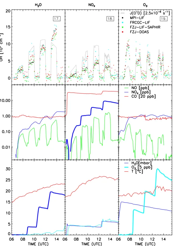
Six days of formal chamber measurements took place from 17–23 July 2005. The first three days were used to test po-tential interferences by humidity, NOx, and O3, respectively
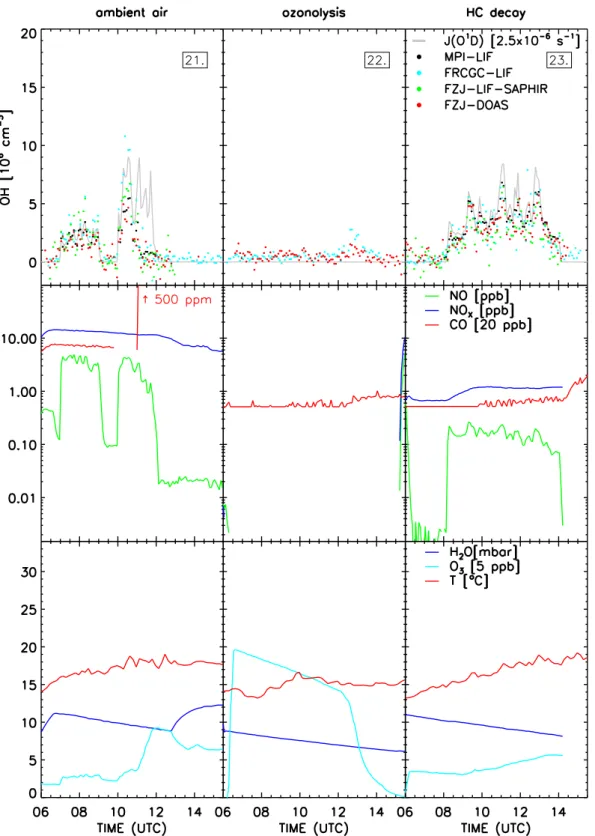
(Fig. 4). The instruments were compared in the chamber flushed with outside air on day 4. The following day was spent to investigate the ozonolysis of alkenes as a radical source in the dark. On the last day, OH was measured during photo-oxidation of a mix of hydrocarbons. Measurements of the last three days (21–23 July 2005) are presented in Fig. 5. 3.4.1 Test for interferences by water vapour
Four humidity levels were tested starting with the flushed, clean, dry chamber at a water vapour partial pressure below 0.07 mbar (dew point−44◦C). Each test phase lasted two hours of which one hour was needed to change the gas mix-ture in the dark and one hour was used to expose the
cham-ber to the sun (see 1st column in Fig. 4). On 17 July 2005 the sky was cloud free and it was very sunny, with moder-ate temperatures (278 K to 295 K). The main source for OH radicals is the photolysis of HONO that is released by the chamber wall. The water dependent HONO source has been described for SAPHIR with a heterogeneous formation term in the dark and a photolytic term (Rohrer et al., 2005). At the beginning of the experiment the HONO concentration was below (3±1) ppt and increased up to approximately 450 ppt for the highest water concentration. Another important rad-ical source is the photolysis of HCHO which is photochem-ically released by the chamber. Its concentration was be-low the detection limit at the beginning of the experiment (<0.07 ppb) and increased to 3 ppb at the end of the exper-iment. The background reactivity of the chamber produced up to 10 ppb O3which is photolysed yielding OH in presence
of water vapour.
In the flushed dark chamber the OH data of all instruments (FRCGC-LIF, FZJ-LIF-SAPHIR, and FZJ-DOAS) scattered around zero within the respective precisions. OH data of all instruments ranged between (2 and 3)×106cm−3during the
60 min of insolation of the first humidity step. After closing the louvre system all instruments detected zero OH in the chamber again. But during the following insolation period at 3.7 mbar H2O (dew point−7◦C) some differences between
the instruments are observed. The FZJ-LIF-SAPHIR and the MPI-LIF measured lower OH level ((4–5)×106cm−3), the FZJ-DOAS slightly higher, and the FRCGC-LIF the highest values ((7–8)×106cm−3). However, for the next humidity level (up to 12.7 mbar H2O, dew point 10◦C) the measured
OH concentrations of all instruments are very similar ((8– 10)×106cm−3). Also for the last step with the highest wa-ter concentration (up to 19.6 mbar H2O, dew point 16◦C) all
instruments show identical OH concentrations within their precision. The highest average OH concentration measured throughout the campaign ((11–15)×106cm−3) was seen
dur-ing this last step despite decreasdur-ing photolysis frequencies because all major OH sources accumulated towards the end of the experiment while the concentration of organic trace gases that react with OH was very low. During the last two irradiation periods the fan was operated for 10 min each (11:10–11:20, 13:40–13:50), but no effect on the OH mea-surements was observed.
3.4.2 Test for interferences by NOx
On 18 July 2005 (2nd column in Fig. 4) (500–800) ppb CO, 20 ppb O3, and (3–6) mbar H2O were added to the
cham-ber in order to assure conditions (background reactivity, hu-midity) that are relevant for field measurements. The NOx
mixing ratio was changed in three steps (<0.22 ppb, 1.1 ppb, 3.5 ppb, and 8.8 ppb). Before the last step CO, O3, and H2O
the experiment. The cycling between dark periods and in-solation followed the scheme of the previous day. However, photolysis frequencies were lower because of a hazy sky and occasional clouds. The average OH concentration was con-siderably lower, mostly below 5×106cm−3as a consequence of the lower insolation, higher reactivity, and lower OH radi-cal sources (less HONO and HCHO, but more O3and H2O).
Like on the previous day, the instruments measured no sig-nificant OH concentrations during the dark periods and agree mostly during the insolation periods. During the last insola-tion period the fan was operated (13:35–13:40, 13:45–13:50, and 13:55–14:00). No change in OH concentration or scat-ter of the data caused by the enforced mixing or induced by the increased turbulence was observed for any of the instru-ments.
3.4.3 Test for interferences by ozone
Ozone was varied between 0 ppb and 150 ppb in steps of 50 ppb on 19 July 2005 (3rd column in Fig. 4). At the begin-ning of the experiment 17 ppb CO was present and 15 mbar H2O was added. NOxwas (0.7–1.0) ppb. This day was partly
cloudy and the temperature varied little (290 K–295 K). The HCHO concentration increased up to 2.9 ppb. The HONO production was first very large and the mixing ratio increased steeply during the first insolation period from 50 ppt to (450– 500) ppt, but then decreased to reach 250 ppt at the end of the experiment.
During the first period, HONO was the most important OH source at a low OH reactivity, therefore the highest OH concentrations up to 10×106cm−3were measured by all
struments. The OH concentration during the following in-solation periods was lower and highly variable because of the variable photolysis frequencies. On this day, the instru-ments show general good agreement within the precision of the data independent of the level of ozone. Interestingly, all instruments measured an increasing OH concentration differ-ent from zero in the dark chamber (no valid data of the MPI-LIF). The average OH concentration in the dark was found to be approximately 1×106cm−3 at the end of the experi-ment. In order to test the contribution of OH produced and detected by the laser beam of the FZJ-DOAS the fan was op-erated during three intervals (07:50–07:55, 09:50–09:55, and 13:40–13:50) in addition to the periods of mixing during O3
addition. But no significant change in the OH concentration was observed. Another test was conducted after the exper-iment by increasing the UV laser power to 4 mW during an interval without fan operation. The OH concentration mea-sured by DOAS increased to maximum 4×106cm−3, there-fore this interference is estimated to have been well below 1×106cm−3during the experiment.
3.4.4 Aging of J ¨ulich ambient air
On 21 July 2005 the dark SAPHIR chamber was flushed with particle filtered ambient air. The intention of this experiment was to compare the OH instruments using outside air without local emissions. As shown in the first column in Fig. 5 the chamber volume was exposed to daylight two times: 07:00– 09:02 and 10:00–12:00. The fan was turned on 10:40–10:50 to test homogeneity within the chamber.
The FZJ-DOAS instrument revealed, in addition to the absorbance by OH and HCHO, significant contributions by 2.5 ppb SO2 and 60 ppt naphthalene (C10H8). Both
com-pounds are markers for fossil fuel combustion by several large, lignite-fired power plants near J¨ulich. Other combus-tion markers include 160 ppb CO and 14 ppb NOx. Benzene
and toluene were about 0.5 ppb each and biogenic VOCs were below 0.2 ppb. HCHO was 1.3 ppb at the beginning of the experiment and increased to 3.3 ppb during the course of the two periods of insolation. The HONO concentration at the beginning of the experiment was approximately 250 ppt and increased to 490 ppt after the first insolation period and then decreased continuously to 290 ppt. Ambient air had 9 ppb O3, which increased up to 47 ppb during the second
insolation. From 11:00 to 11:15, approximately 500 ppm of CO was added in order to completely scavenge OH.
During this mostly cloudy day with temperatures around 290 K the OH measurements were variable and mostly less than 5×106cm−3during the first period of insolation. The FRCGC-LIF detected up to 10×106cm−3of OH during the second insolation period, while other instruments showed approximately 6×106cm−3. After addition of CO the data of the FZJ-DOAS, the FZJ-LIF-SAPHIR, and the FRCGC-LIF are not significantly different from zero, while the data of the MPI-LIF shows a small offset of (7±2)×105cm−3.
The offset showed up during insolation and therefore cannot be explained by the known artefact in the dark. It is likely caused by a small interference to HO2, which is detected in
the MPI-LIF instrument downstream of the OH detection cell by chemical conversion with added NO. Given the high HO2
concentrations of about 6×108cm−3in the SAPHIR cham-ber after CO addition, small amounts of NO contamination, for example, by backdiffusion, may have caused the small offset in the OH measurements. An interference of this mag-nitude, however, has little relevance for atmospheric condi-tions, where HO2/OH ratios are typically 10–100.
3.4.5 Ozonolysis of alkenes
This experiment was designed to form different, nearly con-stant HO2concentration levels by reacting alkenes with O3in
the dark (second column in Fig. 5). Only very small steady-state concentrations of OH are expected, which makes the experiment sensitive to potential interferences due to HO2
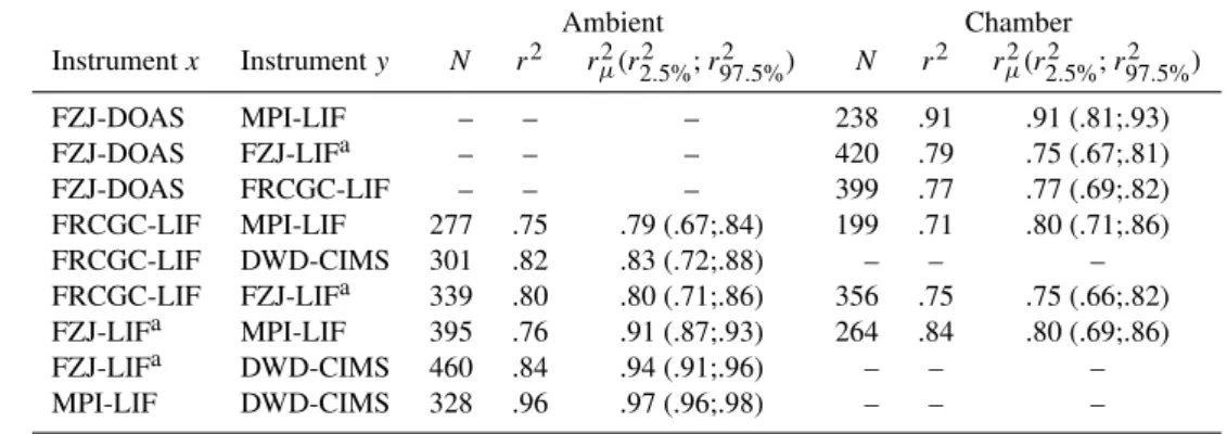
Table 3. Correlation results (r2) of data averaged to common 300 s intervals (number of dataN). The square of the expected correlation coefficientrµ2(2.5% and 97.5% percentiles) was calculated from a-priori stated precision of the individual instruments.
Ambient Chamber
Instrumentx Instrumenty N r2 rµ2(r22.5%;r972.5%) N r2 rµ2(r22.5%;r972.5%)
FZJ-DOAS MPI-LIF – – – 238 .91 .91 (.81;.93) FZJ-DOAS FZJ-LIFa – – – 420 .79 .75 (.67;.81) FZJ-DOAS FRCGC-LIF – – – 399 .77 .77 (.69;.82) FRCGC-LIF MPI-LIF 277 .75 .79 (.67;.84) 199 .71 .80 (.71;.86) FRCGC-LIF DWD-CIMS 301 .82 .83 (.72;.88) – – – FRCGC-LIF FZJ-LIFa 339 .80 .80 (.71;.86) 356 .75 .75 (.66;.82) FZJ-LIFa MPI-LIF 395 .76 .91 (.87;.93) 264 .84 .80 (.69;.86) FZJ-LIFa DWD-CIMS 460 .84 .94 (.91;.96) – – – MPI-LIF DWD-CIMS 328 .96 .97 (.96;.98) – – –
aFZJ-LIF stands for two independent FZJ instruments; ambient: FZJ-LIF-ambient, chamber: FZJ-LIF-SAPHIR.
After the addition of water vapour (9 mbar, dew point 5◦C) and 100 ppb O3 the experiment was started by addition of
6 ppb pent-1-ene at 07:30. Another 15 ppb was added at 09:05 and the last addition of 25 ppb pent-1-ene was at 10:30. A second block of alkene injections followed in order to in-crease the OH yield and to test the upper range of HO2. Four
200 ppb injections of trans-2-butene were applied at 12:08, 12:34, 12:53, and 14:15. There was 70 ppb O3left during the
first injection and O3was titrated by following alkene
addi-tions.
As noted before, only OH data of FRCGC-LIF and FZJ-DOAS can be compared on this day. A potential interfer-ence with O3 of the DOAS instrument (Sect. 2.1.1) was
counteracted by using a low UV laser power and by oper-ation of the fan throughout the experiment. We estimate that it was below 2×105cm−3during this experiment. Very good agreement of OH measured by the two different tech-niques was found. Both instruments reported a non-zero OH concentration of (0.40±0.05)×106cm−3(FRCGC-LIF) and (0.47±0.10)×106cm−3(FZJ-DOAS), before trans-2-butene was added. No change of the OH concentration is observed when pent-1-ene is added and no influence of the increasing HO2 levels is discernable during the first part of the
exper-iment. However, the addition of a large amount of trans-2-butene is reflected by a distinct rise in the OH concentration detected by both instruments. The last addition of alkene did produce no further increase in OH at the end of the ex-periment, because with the titration of O3 the OH
produc-tion ceased. The FRCGC-LIF measured up to 3.0×106cm−3
of OH, while the FZJ-DOAS measured 1.9×106cm−3. Af-ter the last pent-1-ene addition HO2 was in the range of
4×108cm−3. High levels of up to 38×108cm−3were cre-ated as measured by LIF after the third addition of trans-2-butene. The measured HO2/OH ratio was then
approxi-mately 2000. The FRCGC-LIF has an alternating measure-ment of OH and HO2and a tiny NO leak would form OH
from HO2. This might explain the difference to the
FZJ-DOAS measurement. However, it was confirmed during cal-ibration of the FRCGC-LIF that a HO2/OH ratio of up to 500
can be measured without interferences. 3.4.6 Photooxidation of hydrocarbons
OH concentrations were measured in synthetic air with added hydrocarbons, including alkanes, alkenes and aro-matic compounds. The following trace gases were added: water vapour (11 mbar, dew point 10◦C), NO (0.7 ppb),
O3 (17 ppb) and 6 different hydrocarbons (5 ppb benzene,
3 ppb 1-hexene, 2.5 ppbm-xylene, 3 ppbn-octane, 3 ppb n-pentane, and 1 ppb isoprene). The last formal chamber ex-periment is shown in the 3rd column in Fig. 5. Photochem-istry was started by opening the louvre system (08:10), but sunlight was modulated by a broken cloud cover. Initially, up to 350 ppt of HONO were formed that later decreased to 180 ppt. Photooxidation of VOCs resulted in the production of up to 29 ppb O3and 4.3 ppb HCHO. HO2and RO2
mea-sured by LIF and MIESR, respectively, were in the range of (1.5–5.0)×108cm−3. The measurements of all instruments showed good agreement within the precision of the measure-ments in the dark and at daylight.
4 Discussion
4.1 Correlation
Table 4. Result of the regression to the data (300 s mean values): the regression slope (b), the intercept (a, in units of 106cm−3), and the sum of the squared residuals divided by the number of data points (Nχ2
−2) which serves as a measure of the fit quality.b0is the ratio of the mean of two data sets (y/¯ x¯).
Ambient Chamber
Instrumentx Instrumenty b0 b a χ 2
N−2 N b0 b a χ
2
N−2 N
FZJ-DOAS MPI-LIF – – – – 1.00±0.07 0.98±0.02 10.14±0.08 1.3 238 FZJ-DOAS FZJ-LIFa – – – – 0.87±0.07 0.95±0.02 −0.23±0.07 1.3 420 FZJ-DOAS FRCGC-LIF – – – – 1.05±0.09 1.09±0.03 −0.09±0.08 1.1 399 FRCGC-LIF MPI-LIF 1.11±0.06 1.26±0.03 −0.63±0.15 1.3 277 0.89±0.06 1.01±0.03 −0.41±0.17 1.6 199 FRCGC-LIF DWD-CIMS 0.66±0.04 0.75±0.02 −0.31±0.07 1.2 301 – – – – – FRCGC-LIF FZJ-LIFa 0.95±0.06 1.06±0.02 −0.21±0.10 1.4 339 0.82±0.07 0.88±0.03 −0.01±0.09 1.3 356 FZJ-LIFa MPI-LIF 1.19±0.06 1.29±0.01 −0.29±0.06 4.9 395 1.10±0.07 1.10±0.02 10.00±0.10 1.8 264 FZJ-LIFa DWD-CIMS 0.69±0.05 0.70±0.01 −0.04±0.03 4.0 460 – – – – – MPI-LIF DWD-CIMS 0.62±0.03 0.59±0.01 10.08±0.03 1.9 328 – – – – –
aFZJ-LIF stands for two independent FZJ instruments; ambient: FZJ-LIF-ambient, chamber: FZJ-LIF-SAPHIR.
The correlation coefficientsr2of the 300 s-averaged, com-bined data sets in Table 3 range between 0.71 (FRCGC/MPI) and 0.96 (ambient CIMS/MPI), which includes both ambient and chamber measurements. These results indicate that be-tween 71% and 96% of the OH variability measured by all instrument pairs is real. The results are similar for the am-bient and the chamber measurements. The instruments can be ordered from high to lowr2when the possible combina-tions of three instruments pairs are compared: DWD-CIMS, MPI-LIF, FZJ-DOAS, FZJ-LIF-ambient, FZJ-LIF-SAPHIR, FRCGC-LIF. This is basically also the order of the a-priori stated precision of the different instruments, when averaged over a common time step. Experimental data of each instru-ment has a statistical dispersion described by the precision of its OH measurement characteristics. The finite dispersion re-sults in ar2<1.00 even if the variation is entirely explained by the precision. A Monte Carlo analysis was used in or-der to assess the influence of the precision as opposed to other potential nonstatistical errors. 1000 random data sets each were generated to determine the expected valuerµ2 that is likely obtained when a pair of data is identical, but each afflicted with the respective instruments precision that was randomly varied for each data point using a normal distri-bution. Because the resulting distribution is not Gaussian, a Fischer transformation was used to calculate its centre (rµ2) and the 2.5% and 97.5% percentiles that are listed in the third subcolumn of Table 3. The experimental values of r2 are completely in agreement withrµ2within the 2.5% and 97.5% percentiles except for two instrument pairs: The FZJ-LIF-ambient versus the DWD-CIMS and the MPI-LIF, respec-tively.
The lower than expectedr2 of these instrument pairs is possibly caused by an unknown systematic instrumental er-ror or probing of different air influenced by local emissions. The latter possibility is favoured by the distance between the DWD/MPI and FZJ instruments that was larger than for other
instrument combinations. On the other hand, the experimen-talr2of instrument pairs at the chamber is found to be always within the confidence intervals. This suggests that all instru-ments sampled correctly the same OH concentration that is expected in a homogeneous environment as provided by the SAPHIR chamber.
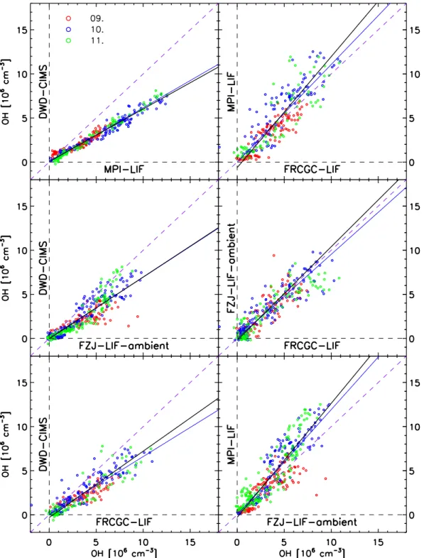
4.2 Regression
Linear regressions (y=a+b·x) were calculated for the six possible instrument combinations of the measurements at the field site and for the six combinations at the SAPHIR chamber. The regressions account for the statistical errors of both instruments (x- andy-axis) based on the algorithm “fi-texy” proposed by Press and Teukolsky (1992). Additionally, the slopes of regressions with the origin forced through zero (y=b0·x) were calculated, whereb0corresponds to the ratio
of the mean OH concentration measured by the respective instruments. The results are shown in Figs. 6 and 7 (without error bars, see Table 2 for average standard deviations) and in Table 4.
The regressions to the ambient data of three days are in general linear (Fig. 6). The regression between MPI-LIF and DWS-CIMS data, upper left panel in Fig. 6 and last row in Table 4, revealed the strongest deviation from unity slope (b=0.59±0.01 andb0=0.62±0.03), although the data
appear negligible in view of the consistent and precise mea-surements throughout the three days of ambient sampling. This implies that the systematic deviation from unity slope is not due to inhomogeneities in the air sampled by either instrument which could be caused by local emissions, but arises from a calibration difference. The deviation from unity slope is just within the limits of the combined cali-bration accuracies specified for the instruments (see Table 1: 32% (MPI) and 38% (DWD)).
The lower precision of the other instruments obscures rel-ative sensitivity trends during the three days, but FZJ-LIF-ambient and FRCGC-LIF compare better than any of their combinations with other instruments: the slope of the re-gressions between FZJ-LIF-ambient and FRCGC-LIF, right panel in the middle row of Fig. 6 and row 6 in Table 4, is unity (b=1.06±0.02 andb0=0.95±0.06) although the data
points are significantly more scattered than those of DWD-CIMS and MPI-LIF which show least agreement on an abso-lute scale. The slopes of all other regressions (see Table 4) are intermediate between these extremes.
Based on this observation and the correlation results, two groups of instruments can be identified that compared well at the field site: On one hand side DWD-CIMS and MPI-LIF, and on the other hand side FRCGC-LIF and FZJ-LIF-ambient. Only systematic inhomogeneities at this site would explain the existence of two distinct groups. Indeed, DWD-CIMS and MPI-LIF were located next to each other (5.5 m, see Fig. 1). FRCGC-LIF neighbored MPI-LIF (3.2 m) and FZJ-LIF-ambient (4.5 m) and both, FRCGC-LIF and FZJ-LIF-ambient, were downwind of the other two instruments. The intercepts of the regression lines are small compared to daytime OH values and range from (−0.04±0.03)×106cm−3 (FZJ-LIF/DWD-CIMS) to
(−0.63±0.15)×106cm−3 (FRCGC-LIF/MPI-LIF). The in-tercepts of some instrument combinations are statistically significant, which may partly result from having two system-atically differing groups of instruments. The slightly larger OH concentration measured by FRCGC-LIF relative to FZJ-LIF-ambient and DWS-CIMS in the night of 10–11 July 2005 (Fig. 3) is another possible contribution. If the regres-sion parameterχ2listed in Table 4 is in the range of the num-ber of data (χ2≈N−2), i.e. the ratioχ2/(N−2)≈1, then the residual variation is explained by the precision of both instru-ments. This is indeed the case for all instruments except for the ambient measurements involving FZJ-LIF-ambient and MPI-LIF or DWD-CIMS (χ2/(N−2)≥4).
For FZJ-LIF-ambient the scatter of the data is not ex-plained by the calculated measurement errors. But it is more in line when FZJ-LIF is compared with FRCGC-LIF, yield-ingχ2/(N−2)=1.4. Most likely this is caused by the sys-tematic difference between the two groups of instruments, in agreement with the findings of the correlation analysis ofr2. The regression analysis of the OH data measured during six days in the SAPHIR chamber indicates very good agree-ment for all OH instruagree-ments for all days (Fig. 7, Table 4). In
fact, the slopes of the regression lines deviate no more than 12% from unity for all instrument combinations, which is better than expected from the stated accuracies.
It should be noted that half of the dynamic OH concentra-tion range is determined by two days (17 and 19 July 2005). Data of 22 July 2005 is missing for all instrument pairs ex-cept for FZJ-DOAS and FRCGC-LIF. The slopes (bandb0)
calculated for chamber data of all six days agree within the error margins for all instruments, suggesting negligible off-sets between different instruments. This is also demonstrated by the calculated intercepts of the regression lines which are not significantly different from zero. The values calculated forχ2/(N−2)are 1.1 to 1.8 and good for experimental data. The residual variation is mostly explained by the measure-ment errors and the OH data sets agree quantitatively. This implies that the instruments sampled the same OH concen-tration and it also demonstrates that SAPHIR offers a homo-geneous air composition suitable for instrumental intercom-parisons.
4.3 Comparison of ambient and chamber results
Few instruments provided data that allows to compare the results from the ambient and chamber intercomparisons. MPI-LIF and FRCGC-LIF were the only instruments that measured both in ambient and chamber air. Furthermore, FZJ-LIF-ambient and FZJ-LIF-SAPHIR, which are techni-cally similar and share the same calibration unit, measured in ambient and chamber air, respectively. All LIF instru-ments showed very good agreement among each other in the SAPHIR chamber and in comparison with the calibration-independent DOAS instrument. In ambient air, however, the slope of FRCGC-LIF/MPI-LIF was larger by 25% than in the chamber, the slope of FZJ-LIF/MPI-LIF larger by about 17%, while the corresponding slope of FRCGC-LIF/FZJ-LIF was larger by about 20%. As discussed before, inhomoge-neous air has probably influenced the slopes of MPI-LIF ver-sus FRCGC-LIF and FZJ-LIF in ambient air, but there is no such indication for FRCGC-LIF versus FZJ-LIF. This sug-gests that sensitivity changes may have occurred in ambient air for the LIF instruments, which may be in the order of 20% and are not accounted for by the calibration procedures. It is not possible to resolve the differences between the OH measurements in ambient air since no ambient DOAS mea-surements are available as absolute reference.
4.4 Interferences
H2O, O3, NOx, ROx, and VOCs. The FZJ-DOAS data was
chosen as reference because of its high accuracy.
Since the chemical conditions inside the chamber were changed in the periods when the louvre system was closed, measurements during these periods were excluded from this analysis. The residuum values (1OH) of the regression of LIF versus DOAS data, OH, were binned for each insola-tion period and plotted as a funcinsola-tion of the corresponding concentrations of H2O, NOx, O3, HO2 (Fig. 8). The
min-imum, 25%-quartile, median, 75%-quartile, and maximum were calculated for each bin and are presented as box whisker plots. Positive values of 1OH indicate that a LIF instru-ment measured relatively higher OH concentrations than the DOAS instrument.
The plots of the first column of Fig. 8 show the analysis with respect to different absolute humidity levels. The scat-ter of1OH is large because of the combined precision of two instruments. For all, but the second humidity level (3.6 mbar H2O) no large deviation is found. Compared to the DOAS
measurement, the MPI-LIF measured systematically lower OH concentrations (−1.6×106cm−3) whereas the FRCGC-LIF measured 1.2×106cm−3higher OH concentrations for the same humidity level. This deviation is unexpected, be-cause it is unrelated to the water concentration and bebe-cause inhomogeneity inside the chamber is unlikely. Therefore, it must be attributed to a temporal instability of the OH sensi-tivity of these two instruments. Overall, no systematic trend regarding a potential cross sensitivity to water vapour is ob-served. The OH sensitivity of the LIF instruments was suc-cessfully corrected for the increase in the quenching rate by increasing mixing ratios of water vapour.
The differences between DOAS and LIF are investigated with regard to different NOx levels as shown in the second
column of Fig. 8. The OH concentrations of this cross sensi-tivity test were lower than for the other tests. The data does not reveal any trends and no cross sensitivity to NOxon the
measurements of any instrument can be detected.
OH interference by laser photolysis of ozone has been a se-vere problem in atmospheric OH measurements in the past (Smith and Crosley, 1990), but is assumed to be essentially eliminated in current OH laser instruments. This is con-firmed by a corresponding interference test on the third day of chamber experiments (see Sect. 3.4.3). Figure 8 shows no significant differences between the LIF instruments and DOAS, and no trend is observed even when ozone was in-creased up to 143 ppb.
The experiment with ambient air was used to investigate a potential HO2 interference. During the second part of
the experiment CO was added to scavenge OH and pro-duce HO2. Only two bins were used here, the first one with
HO2concentrations below 0.5×108cm−3, the second one at
(6±2)×108cm−3. The MPI-LIF did measure OH concen-trations(7±2)×105cm−3after the addition of CO in order to completely scavenge OH, as discussed in Sect. 3.4.4. But considering the precision of this analysis, this potential
in-Fig. 8. The residual differences of OH data measured by the three different LIF instruments and FZJ-DOAS versus variable water vapour, NOx, O3, and HO2concentrations. The box whisker plots indicate minimum, 25%-quartile, median, 75%-quartile, and maxi-mum.
terference cannot be confirmed. For none of the LIF instru-ments a significant influence of the HO2concentration on the
OH measurement can be detected for conditions relevant for the atmosphere.
5 Conclusions
HOxComp was the first formal, blind intercomparison cam-paign of OH measurements which involved six differ-ent instrumdiffer-ents (4 LIF, 1 CIMS, and 1 DOAS) operated by Japanese and German groups. It covered three days of mea-surements in ambient air and six days of meamea-surements in the atmosphere simulation chamber SAPHIR. The ambient con-ditions were moderately polluted with substantial levels of biogenic VOCs. In this work we attained a number of find-ings which we think are of importance for the interpretation of past, present, and future OH measurements: