Random resistivity network calculations for cuprate superconductors with an electronic phase separation transition

(1)

Contents lists available atSciVerse ScienceDirect

Physica A

journal homepage:www.elsevier.com/locate/physa

Random resistivity network calculations for cuprate superconductors

with an electronic phase separation transition

C.F.S. Pinheiro

a

, E.V.L. de Mello

b,∗

a_{Centro de Pesquisa de Tecnologia Nuclear, Belo Horizonte, MG 31270-901, Brazil} b_{Instituto de Física, Universidade Federal Fluminense, Niterói, RJ 24210-340, Brazil}

a r t i c l e i n f o

Article history:

Received 17 June 2011

Received in revised form 12 August 2011 Available online 6 September 2011

Keywords:

Random resistivity network Phase separation transition Superconductor transition High critical temperature transition

a b s t r a c t

The resistivity as a function of temperature for high temperature superconductors is very unusual and, despite its importance, lacks a unified theoretical explanation. It is linear with the temperature for overdoped compounds but it falls more quickly as the doping level decreases. The resistivity of underdoped cuprates increases like that of an insulator below a characteristic temperature where it shows a minimum. We show that this overall behavior can be explained by calculations using an electronic phase segregation into two main component phases with low and highelectronic densities. The total resistance is calculated from the various contributions through several processes of random picking of the local resistivities and using a common statistical random resistor network approach.

1. Introduction

The nature of the underlying mechanism governing the high critical temperature superconductors (HTSC) has become one of the most studied problems in condensed matter physics. Despite the intensive experimental and theoretical effort, there is no consensus on the basic mechanism or on the generic phase diagram. In contrast to the normal phase of the low temperature superconductors, which is the well known Fermi liquid, that of HTSC has many properties that are not understood and not Fermi liquid like. For instance, HTSC have a normal-state gap or pseudogap that in some cases persists at temperatures much higher than the resistivity transition temperatureTc[1] and whose origin is still a matter of great debate. The pseudogap manifests itself by a suppression of the spectral weight of the normal-state electronic density of states as established by many different experiments on bulk and surfaces, and momentum and real space, as has been extensively discussed in many review articles [1–3]. Consequently, it has become accepted that the HTSC phase diagram is dominated by two energy scales and two distinct forms of quasiparticle dynamics [3,4], one associated with the superconducting phase the other associated with the pseudogap temperatureT∗_.

Another important feature of the cuprate superconductors is the presence of inhomogeneities. A phase separation transi-tion was observed experimentally a long time ago in La2CuO4₊y[5]. In that experiment the phase separation of the interstitial oxygens is accompanied by an electronic phase separation of holes in CuO2planes. Many different experiments have added evidence that the charge distribution in the CuO2planes of the high temperature superconductors (HTSC) is microscopically inhomogeneous—for example, neutron diffraction [6,7], muon spin relaxation (

µ

SR) [8], NQR and NMR [9,10] studies. These experiments indicated that the inhomogeneities are more pronounced on the underdoped side of the phase diagram and related this to the non-Fermi liquid behavior of the normal phase. Recent scanning tunneling microscopy (STM) studies on Bi2212 revealed spatial variations of the electronic gap amplitude on a nanometer length scale even for overdoped com-pounds [11–13]. The local density of states (LDOS) measured in these STM experiments [11–13] has two different forms that

∗Corresponding author. Tel.: +55 21 26295822.

(2)

are possibly associated with a segregation into metallic and insulator nanoscopic regions [14]. Consequently the electronic phase separation in cuprates has been the subject of many articles [15–22] and many books [23–25].

The electronic disorder of the normal phase is manifested in many transport properties of a HTSC series, like the resistivity as a function of the temperatureR

(

T

)

, which, despite its importance, lacks a widely accepted explanation. Here we want to show that the particular behavior ofR

(

T

)

for different compounds of a single series is a manifestation of the intrinsic inhomogeneity of these materials. We can divide the resistivity behaviors for a system into three general kinds, as follows. It falls linearly with the temperature for samples in the overdoped regions [26]. It falls below the linear trend for compounds near the optimum values, as measured by several groups [27,28]. For very low doping it falls with the temperature, reaches a minimum at an intermediate temperature, starts to increase at lower temperature until it reaches a local maximum, and then drops to zero belowTc. This reentrant behavior is observed in almost all underdoped cuprates [29–31] but its origin has not been very much discussed in the literature. The significance and origin of such rich phenomena will be the focus of our work.

On the basis of the above facts we perform calculations taking into account the EPS transition by the use of the general phase separation theory of Cahn and Hilliard (CH) [32]. It describes how a system evolves from small fluctuations around an average densitypto a complete separation into low and high density regions. For each of these small regions we will associate a local resistivity derived from the work of Takagi et al. [26], who performed systematic measurements on the LSCO series (La2−pSrpCuO4), with a large range of values ofTandp. Then we use the random resistor network (RRN) method [33] to derive the system resistivity as a function of the temperatureR

(

T

)

in a similar way to how that for the manganites was derived [34]. The local density and resistivity are randomly picked and the finalR

(

T

)

result is an average over many different configurations. We show that the non-conventional features discussed in the previous paragraph are well described by this approach.

2. Electronic phase separation

The electronic phase separation was found by several HTSC experiments and detected to be in the form of either stripes [6,35], a patchwork [36] or a checkerboard [37]. Earlier it was believed that the underlying mechanism of electronic phase separation was associated with defects, or oxygen or cation disorder. Indeed, oxygen phase segregation was observed for La2CuO4+δby means of X-ray and transport measurements [15,5]. However, depending on the type of experiment, there

are some HTSC materials, in particular YBCO, that appear to be more homogeneous or, at least, do not display any gross inhomogeneity [38,39].

On the other hand, electronic phase separation appears to be a universal feature of HTSC. It is seen in the entire series of LSCO by means of neutron diffraction [7] and in many BSCO samples by STM [11–13]. ARPES has also been used to detect distinct quasiparticle behavior in LSCO and BSCO. Recently, inhomogeneous magnetic field response measurements on some LSCO compounds and on the YBa2Cu3Oy(YBCO) family [40] were also interpreted as compatible with electronic phase separation, forming domains. Particularly in the case of YBCO, where doping occurs via a change in the oxygen concentration of the CuO chain, the inhomogeneities cannot be attributed to disorder in the cation substitution, providing strong support for an intrinsic EPS transition. The effect of the annealing time, connected to the structural organization of oxygen interstitials, for La2CuO4₋ywas studied recently using X-ray diffraction techniques [22]

The possible origin of this EPS transition is the proximity to the insulator AF phase, common to all cuprates, as we derived from the principle of the competing minimum free energies [19]. These calculations yield a lineTPS

(

p

)

close to the experimental results reported by Timusk and Statt [1] (T0_{in their notation), and this has been taken as a linear function} just for simplicity, as is schematically shown inFigs. 2 and4. When the temperature decreases belowTPS

(

p

)

, the free energy of the homogeneous system with average densitypbecomes lower than the anisotropic one derived from a bimodal distribution [16] of AF domains withp

(

i

)

≈

0 and high hole density domains withp

(

i

)

≈

2p. This approach is justified by the NQR experimental data [9] which were interpreted as coming from two distinct regions with symmetric local doping around the average valuep. The two symmetrical local dopings increase their differences as the temperature is lowered, which is characteristic of second-order transitions.

To describe the formation of the local hole density domains we define the difference between the local and the average charge densityu

(

i

,

T

)

≡

(

p

(

i

,

T

)

−

p

)

as the EPS transition order parameter. Clearlyu

(

i

,

T

)

=

0 corresponds to the homogeneous system aboveTPS

(

p

)

. Then the typical Ginzburg–Landau free energy functional in terms of such an order parameter near the transition is given by

f

(

i

,

T

)

=

1 2

ε

2

|∇

u

(

i

,

T

)

|

2

+

V

(

u

(

i

,

T

))

(1)

where the potentialV

(

u

,

T

)

=

A2

(

T

)

u2

/

2

+

B2u4

/

4

+ · · ·

,A2

(

T

)

=

α(

TPS

(

p

)

−

T

)

, and

α

andBare constants that lead to lines of constant values ofA

(

T

)/

B, parallel toTPS

(

p

)

, as shown inFig. 1.

ε

gives the size of the grain boundaries among two low and high density phasesp_±

(

i

)

[41,17]. The energy barrier between two grains of distinct phases isEg

(

T

)

=

A4

(

T

)/

B, which is proportional to

(

TPS

−

T

)

2near the transition, and becomes nearly constant at low temperatures. The two minima ofV

(

u

,

T

)

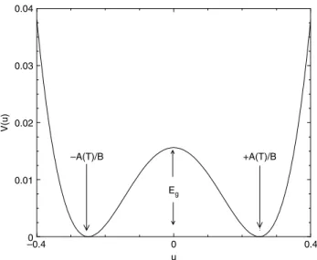
are shown inFig. 1.

(3)

–0.4 0 0.4 u

0 0.01 0.02 0.03 0.04

V(u)

–A(T)/B

Eg

+A(T)/B

Fig. 1. The potential commonly used in the free energy of the CH equation which gives rise to phase separation as a function of the order parameteruor the densityp. Notice that the two minima yield the two equilibrium low and high density phases and the energy barrier or free energy wallEgdepends on how far the temperature is belowTps, that is, the temperature differenceTps−T.

are parallel toTPS

(

p

)

. InFig. 2we plotTPS

(

p

)

where the phase separation starts,T0

(

p

)

where the EPS is detected andT1

(

P

)

where insulator grains appear, all assumed to be linear inpjust for simplicity, but in agreement with some signals detected by many experiments [1–4]. DM and DI are phases with low disorder in the sense that the two phases are metallic (DM) or insulator (DI). At lower temperatures, the disorder increases and the system is composed of very low density or insulator regions and very high density or metallic regions (DM

₊

DI). SeeFig. 2.

The CH equation can be written [42] in the form of a continuity equation of the local density of free energyf,

∂

tu

= −

∇

·

J, with the currentJ

₌

M

∇

(δ

f

/δ

u

)

, whereMis the mobility or the charge transport coefficient. Therefore,

∂

u

∂

t

= −

M

∇

2

_(ε

2

∇

2u

+

A2

(

T

)

u

−

B2u3

).

(2)

In previous papers we have verified the applicability of the CH approach [41]. We have made a detailed study of the density profile evolution in a 105

×

105 array as a function of the time steps, up to the stabilization of the local densities, for parameters that yield stripe [18] and patchwork [17,43] patterns.

Here we want to concentrate on the energy structure of the grains which leads to additional scattering and changes the whole charge dynamics. We show that belowTPS, the grain boundary energiesEg (see the inset ofFig. 2) increase as the temperature goes down, segregating and confining holes to certain regions or grains with an increasing difference in the local doping. The confining potential favors pair formation at low temperatures, giving rise to the local superconductivity in isolated regions.

As the temperature goes down below theTPS

(

p

)

, the system increases the phase separation and in favorable conditions tends to form a bimodal distribution made up of low and high density domains.Fig. 2shows the various levels of phase separation as a function of the temperature difference

|

TPS

−

T

|

. At low density (p

≤

0

.

16) and low temperature the system can achieve the maximum charge segregation and become composed essentially of phases of two densities, one withp

(

i

)

≈

0 and the other withp

(

i

)

≈

2p. There are disordered insulator (DI) regions and disordered metallic (DM) ones. InFig. 3we show this situation for the case withp

=

0

.

16 andT

≈

0 K, with half of the sites withp

(

i

)

≈

0 and the other half withp

(

i

)

≈

0

.

32, as is seen in the inset histogram for over all the sitesiof the system.

The density map shown inFig. 3is made on a 100

_×

100 unit cell square lattice; the low and high density grains have different sizes and are composed by 30–100 cells. The inset shows the histogram of the local doping at each crystalline site, which shows how the density segregates into two main bands whose width values depend on the temperature.

At low temperatures belowT0

(

p

)

(seeFig. 2), we can consider the grains as isolated entities with very weak intergrain coupling, and a typical Fermi energy of a grain is much smaller than the bulk Debye energy—the so called anti-adiabatic regime [44].

Thus below theT0line inFig. 2, a cuprate is composed of a mixture of insulator (p

(

i

)

≈

0) and metallic (p

(

i

)

≈

2p) grains. A clear experimental realization of such a system is the granular Pb film on a glass substrate which can change from showing insulator behavior to showing superconducting behavior with increasing Pb grain size [45]. For very low average doping the system is mainly insulator, but forp

≥

0

.

05 the large density grains become metallic like, and in general both kinds of regions are present in one single sample.

(4)

1000

800

600

Temperature (K)

400

200

0

0 0.05 0.1 0.15 0.2 Hole Doping p

0.25 0.3 0.35 0.4 DI

DI+DM

DI+DM DM1+DM2 DM TPS

T0 T₁

Fig. 2. Important crossover lines derived from many experiments [1] that are associated with the degree of phase separation. The electronic segregation starts atTPS(p), resulting into two kinds of phases, with high and low densities, as a consequence of the potential shown inFig. 1. DI and DM stand for disordered insulator and disordered metal phases. DI+DM stands for a larger disorder with insulator and metallic phases coexisting. DM1+DM2is the situation in which both phases are metallic, but with different densities.

0 0 50 100 150 200 250

Count

300 350 400 450

0.05 0.1 0.15 local hole density p(i) Local Density Distribution

A(t)/B=1.0, p=0.16

0.2 0.25 0.3

0.841

0.527

0.214

–0.099

–0.413

–0.727

–1.04 0.35

Fig. 3. (Color online) Density map of the system at low temperatures. The low and high density domains are clearly formed. The inset shows the local densityp(i)histogram with average hole densityp=0.16, showing that the high density grains are metallic like and the low density (insulator) ones have

p(i)≈0.

granular superconductors [45]. And the zero-resistivity transition takes place only when the Josephson couplingEJamong these grains is sufficiently large to overcome thermal fluctuations [45], that is,EJ

(

p

,

T

=

Tc

)

≈

kBTc

(

p

)

, which leads to phase locking and long range phase coherence.

In the next section we will use the above results to calculate the average resistivity. The main point is that any compound of a HTSC system goes through EPS transitions and the local densities follow a bimodal distribution with a dispersion similar to that shown in the inset histogram ofFig. 3. This is interpreted as a distribution of local resistivities and will be used in connection with the RRN [33].

3. The resistivity calculations

(5)

PS 600

500

400

300

T

(K)

200

100

0

0 0.04 0.08 0.12 0.16 p

0.2 0.24 0.28 p

δ δ_p

p ∆

Ton

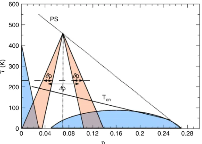
Fig. 4. (Color online) Schematic phase diagram showing the EPS with bands of doping fractionsδp(i)as a function of temperature. At low temperature, belowTon, tiny domains of SC appear in the band on the right, and for low doping compounds small domains of AF insulators appear in the band on the left inside the sample.

nominal doping composition. Two bus bars are imagined to be placed at the top and bottom of the array so that an external voltage source can set a voltage dropV across the network. The total resistivity will be simply obtained as the ratioV

/

I whereIis the total current through the circuit.

As we discussed in the previous section, above the phase separation line (PS), the system has only metallic links, and resistance is considered to be a linear function of temperature. Below PS, phase separation begins and two bands of compositionpare allowed. These bands have their central values∆papart and are

δ

p

(

i

)

wide. Both∆p

(

i

)

and

δ

p

(

i

)

depend on the temperature and are symmetric with respect to the nominal or average compositionp. InFig. 4the bands are drawn in a schematic phase diagram for a nominal doping fractionp

=

0

.

07. The temperature evolution of these bands follows that in the study of the histograms at different temperatures, such as the one shown in the inset ofFig. 3.

Resistivity is a function of both composition and temperature. From the results of Takagi et al. [26], for various compositionspand a given temperature, is possible to devise a nearly exponential dependence on the composition. The metallic links in the RRN will then follow a random distribution in the allowed values ofp

(

i

)

(the bands) and their resistances will be given by a function derived from the values of Takagi et al. [26]:

R

(

p

(

i

),

T

)

=

A

(

T

)

exp

{−

B

(

p

(

i

)

−

p

)

}

(3)

whereB

(

T

)

=

0

.

05 andA

(

T

)

are derived directly from the LSCO series measurements [26].

On the other hand, following experimental results [13,28,45] and calculations [19,16] similar to those for the intragrain superconductivity discussed in the previous sections, some superconducting regions appear at low temperature. Thus, as the temperature decreases belowTon

(

p

)

, a fraction of the most conducting metallic links (largestp

(

i

)

’s) are replaced by SC links and this fraction reaches 100% of the metallic band atTc

(

p

)

. Similarly, insulators appear in the low density band asp

→

0, which happens at lower temperatures, as can be seen inFig. 4. Like the CH phase separation calculations shown in the pre-vious section, the resistivity calculations were made on 100

_×

100 lattices. Periodic boundary conditions were used only on the sides without theVsource terminals. The resulting linear systems that come from Kirchhoff laws were solved with the aid of the subroutine

ma57

_{, provided by HSL, which makes use of a multifrontal algorithm [}₄₇_{], which speeded up the}

calculations. For each value ofpandT we use 300 samples in order to obtain results independent of the random process of sharing thep

(

i

)

distribution. Results of simulations for typical samples near optimum doping are shown inFig. 5for the com-pound Y0.80Ca0.20Ba2Cu3O7−δwith nominal dopingp

=

0

.

136. 300 samples were used for each point in the graph. The phase

separation begins at 400 K; SC links of resistivity 1

_×

10−8_m_Ω_{cm are introduced below 180 K, according to the}_T

on

(

p

)

line. The small error bars tell us how reliable the results are, that is, a very small dispersion is attained with averages made over 300 configurations. It is also remarkable how the

ρ

×

T linear dependence is attained in the calculations with the two-band scenario. That can be explained by the proper choice of the functionR

(

p

,

T

)

defined in Eq.(3), which can be better understood in the light of results obtained by Costa et al. who used renormalization group theory to study a square RRN [48]. For a square RRN having resistors of only two conductivity valuesg1andg2, distributed with probabilitiesq

−

1 andq, respectively, Costa et al. showed that the network overall conductance, expressed as a function of probabilityq, is

σ (

q

)

σ (

1

)

σ (

1

₋

q

)

σ (

1

)

=

g1

g2

.

(4)

With equal probabilities, i.e.q

₌

0

.

5, its overall resistance will simply be

(6)

0 100 200 300 T (K)

0 0.5 1 1.5

ρ

(m

Ω

cm)

Naqib, 2005 simulation RRN

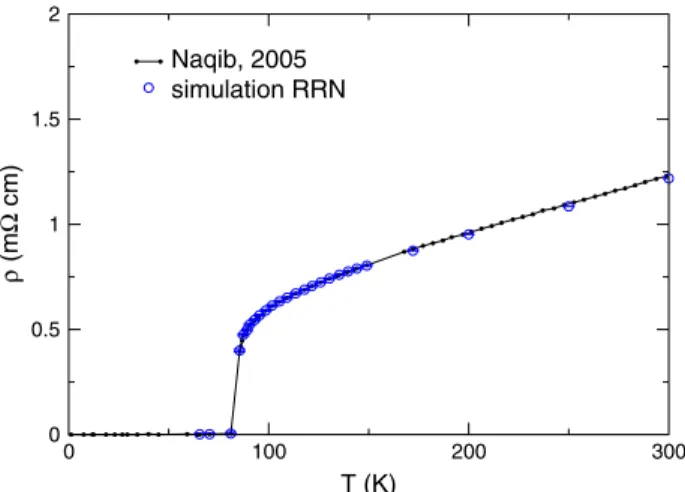
Fig. 5. (Color online) Simulation results compared with experimental data for the case Y0.80Ca0.20Ba2Cu3O7−δwith average dopingp=0.136. As the temperature decreases belowTon=160 K some of the resistance becomes superconducting and the total resistivity decreases below the linear regime. An average over 300 samples was used for each point in the graph.

0 100 200 300 400 500

T (K) 0

1 2 3 4 5 6

ρ

(m

Ω

cm)

Takagi et al. simulated

Fig. 6. Simulation results (circles) for in-plane resistivity of La2₋pSrpCuO4withp=0.07 and the reentrant behavior. Each calculated point is the average over 600 configurations. Dots represent experimental data obtained by Takagi et al. [26].

In our case, if the widths

δ

pare chosen to be zero, a network of links with resistancesR

(

p

−

∆p

(

i

),

T

)

andR

(

p

+

∆p

(

i

),

T

)

would result in an overall resistanceR

(

T

)

=

A

(

T

)

, easily derived from Eqs.(3)and(5). The same result holds for finite width

δ

p

(

i

)

, if symmetric distributions aroundpare used. MakingA

(

T

)

linear is then the right choice. Departures from this linear behavior are explained by the growth of SC and AF domains.

The exact linear dependence ofA

(

T

)

for a given doping fractionpcan be extracted from the linear part of the experimental curves as inFigs. 5and6.

The fraction of SC links to be inserted belowTonwas also calculated from Eq.(4), as follows. The difference between functionA

(

T

)

and the experimental data was normalized byA

(

T

)

itself, and Eq.(4)gave the probabilityqassociated with a network of conductancesg1

=

1 andg2

= [

1

×

10−8mΩcm

]

−1. When distributingp

(

i

)

in the allowed bands by means of random numbersx, uniformly distributed in the interval

_[

0

,

1

_]

, those links for whichx

> (

1

₋

q

)

(the best conductors) were made superconductors.

The resistivity for low doping materials requires special care because it may contain insulator, metallic and superconducting regions represented by links in the RRN method. Thus simulations for a case in which reentrant behavior is present were made for thep

=

0

.

07 compound and the results are shown inFig. 6. We find that such complex behavior is due to the mixture of superconducting and insulator regions in the two different bands. The appearance of the insulator regions in our RRN matrix occurs when

δ

p

(

i

)

crosses the value ofp

(

i

)

≤

0

.

05 [31] at low temperatures, as is demonstrated inFig. 6. This is why, at low temperatures, the resistivity increases, but eventually, as the temperature decreases further and crossesTon, the metallic resistors become superconductors and the resistivity vanishes due to the percolation among the superconducting regions, as we explain below.

(7)

were first added at 140 K asp

(

i

)

reaches the value 0.05 in the low density band. In this case, due to the low values of the densities, the number of samples for each point was 600 for temperatures below 60 K and 300 for the remaining temperatures. AsT

_→

0 both insulating and SC link fractions come close to the link percolation threshold 0.50. That is the reason for the strong variation expressed in the error bars asT

→

0 inFig. 6.

4. Conclusion

In this paper we derived the resistivity of a complete HTSC series assuming an EPS transition. Following many experimental results, we took into consideration that a HTSC compound undergoes an electronic segregation and is composed mainly of two kinds of regions or grains. These are the high and low local density cases, which give a metallic or insulator behavior for the grains as observed from the STM measurements of the LDOS. We used simulations with the CH theory to follow the effects of the EPS as a function of the temperature in order to describe the disordered composition of a HTSC sample.

With this approach, the overall resistivity can be calculated through the RRN method [33] and used to reproduce the measured values in either the overdoped or the underdoped regions. Our method based on the effects of disorder gives results in very good agreement with the measured departure of the linear behavior of near optimum compounds and the completely different down and up reentrant behavior for weakly doped samples that have been studied in detail [31], but so far without a simple and unified interpretation.

The excellent fitting on such a rich variety of features with one single approach without adjustable parameters, and with values of the local resistivities taken from the measurements of Takagi et al. [26] for an entire series, allowed us to conclude the following: the EPS described here and the onset of local or intragrain superconductivity given by the curveTonare universal properties and must be considered to interpret the transport properties of any HTSC system.

Acknowledgments

We gratefully acknowledge partial financial aid from the Brazilian agencies CNPq and Capes.

References

[1] T. Timusk, B. Statt, Rep. Prog. Phys. 62 (1999) 61. [2] J.L. Tallon, J.W. Loram, Physica C 349 (2001) 53.

[3] S. Huffner, M.A. Hossain, A. Damascelli, G.A. Sawatzky, Rep. Prog. Phys. 71 (2008) 062501. [4] M. Le Tacon, A. Sacuto, A. Georges, G. Kotliar, Y. Gallais, D. Colson, A. Forget, Nat. Phys. 2 (2006) 537.

[5] J.D. Jorgensen, B. Dabrowski, Shiyou Pei, D.G. Hinks, L. Soderholm, B. Morosin, J.E. Schirber, E.L. Venturini, D.S. Ginley, Phys. Rev. B38 (1988) 11337. [6] J.M. Tranquada, B.J. Sternlieb, J.D. Axe, Y. Nakamura, S. Uchida, Nature London 375 (1995) 561.

[7] E.S. Bozin, G.H. Kwei, H. Takagi, S.J.L. Billinge, Phys. Rev. Lett. 84 (2000) 5856. [8] Y.J. Uemura, Sol. St. Phys. 126 (2003) 23.

[9] P.M. Singer, A.W. Hunt, T. Imai, Phys. Rev. Lett. 88 (2002) 47602.

[10] H.-J. Grafe, N.J. Curro, M. Hücker, B. Büchner, Phys. Rev. Lett. 96 (2006) 017002.

[11] K. McElroy, D.-H. Lee, J.E. Hoffman, K.M. Lang, E.W. Hudson, H. Eisaki, S. Uchida, J. Lee, J.C. Davis, Phys. Rev. Lett. 94 (2005) 197005. cond-mat/0404005. [12] Kenjiro K. Gomes, Abhay N. Pasupathy, Aakash Pushp, Shimpei Ono, Yoichi Ando, Ali Yazdani, Nature 447 (2007) 569.

[13] Abhay N. Pasupathy, Kenjiro K. Gomes, Colin V. Parker, Jinsheng Wen, Zhijun Xu, Genda Gu, Shimpei Ono, Yoichi Ando, Ali Yazdani, Science 320 (2008) 196.

[14] E.V.L. de Mello, R.B. Kasal, J. Supercond. Nov. Magn. 24 (2011) 1123.

[15] J.C. Grenier, N. Lagueyte, A. Wattiaux, J.P. Doumerc, P. Dordor, J. Etourneau, M. Puchard, J.B. Goodenough, J.S. Zhou, Phys. C202 (1992) 209. [16] E.V.L. de Mello, E.S. Caixeiro, J.L. González, Phys. Rev. B67 (2003) 024502.

[17] E.V.L. de Mello, E.S. Caixeiro, Phys. Rev. B70 (2004) 224517. [18] E.V.L. de Mello, D.N. Dias, J. Phys.: Condens. Matter 19 (2007) 086218.

[19] E.V.L. de Mello, R.B. Kasal, C.A.C. Passos, J. Phys.: Condens. Matter 21 (2009) 235701. [20] D. Innocenti, et al., J. Supercond. Nov. Magn. 22 (2009) 529.

[21] K.I. Kugel, et al., Phys. Rev. B78 (2008) 165124.

[22] M. Fratini, N. Poccia, A. Ricci, G. Campi, M. Burghammer, G. Aeppli, A. Bianconi, Nature 466 (2010) 841. [23] E. Sigmund, K.A. Muller (Eds.), Phase Separation in Cuprate Superconductors, Springer-Verlag, Berlin, 1994. [24] N.L. Saini, in: A. Bianconi (Ed.), Stripes and Related Phenomena, Academic/Plenum publisher, New York, 2000.

[25] A. Bianconi (Ed.), Symmetry and heterogeneity in high temperature superconductors, in: Nato Science Series II, Springer Dordrecht, Netherlands, 2006.

[26] H. Takagi, et al., Phys. Rev. Lett. 69 (1992) 2975. [27] S.H. Naqib, et al., Phys. Rev. B71 (2005) 054502.

[28] C.A. Passos, M.T. Orlando, J.L. Passamai, E.V. de Mello, H.P. Correa, L.G. Martinez, Phys. Rev. B74 (2006) 094514. [29] Y. Ando, et al., Phys. Rev. Lett. 75 (1995) 4662.

[30] S. Ono, et al., Phys. Rev. Lett. 85 (2000) 638.

[31] Seongshik Oh, et al., Phys. Rev. Lett. 96 (2006) 107003. [32] J.W. Cahn, J.E. Hilliard, J. Chem. Phys. 28 (1958) 258. [33] S. Kirkpatrick, Rev. Mod. Phys. 45 (1973) 574.

[34] Matthias Mayr, Adriana Moreo, Jose A. Vergilio, Jeanette Arispe, Adrian Feiguin, Elbio Dagotto, Phys. Rev. Lett. 86 (2001) 135. [35] A. Bianconi, N.L. Saini, A. Lanzara, M. Missori, T. Rossetti, H. Oyanagi, H. Yamaguchi, K. Oda, T. Ito, Phys. Rev. Lett. 76 (1996) 3412. [36] S.H. Pan, et al., Nature 413 (2001) 282–285. and cond-mat/0107347.

[37] T. Hanaguri, C. Lupien, Y. Kohsaka, D.-H. Lee, M. Azuma, M. Takano, H. Takagi, J.C. Davis, Nature 430 (2004) 1001.

[38] J. Bobroff, H. Alloul, S. Ouazi, P. Mendels, A. Mahajan, N. Blanchard, G. Collin, V. Guillen, J.-F. Marucco, Phys. Rev. Lett. 89 (2002) 157002. [39] J.W. Loram, J.L. Tallon, W.Y. Liang, Phys. Rev. B69 (2004) 060502.

(8)

[41] E.V.L de Mello, Otton T. da Silveira Filho, Physica A347 (2005) 429. [42] A.J. Bray, Adv. Phys. 43 (1994) 347.

[43] E.V.L. de Mello, R.B. Kasal, C.A.C. Passos, Otton T.S. Filho, Physica B404 (2009) 3119. [44] E.V.L. de Mello, J. Ranninger, Phys. Rev. B55 (1997) 14872.

[45] L. Merchant, J. Ostrick, R.P. Barber Jr., R.C. Dynes, Phys. Rev. B63 (2001) 134508. [46] J.S. Andrade Jr., N. Ito, Y. Shibusa, Phys. Rev. B 54 (1996) 3910.

[47] I.S. Duff, ACM Trans. Math. Softw. 30 (2004) 118–144.