Fractal analysis of agricultural nozzles spray
Francisco Agüera1*, David Nuyttens2, Fernando Carvajal1, Julián Sánchez-Hermosilla1
ABSTRACT: Fractal scaling of the exponential type is used to establish the cumulative volume (V) distribution applied through agricultural spray nozzles in size x droplets, smaller than the char-acteristic size X. From exponent d, we deduced the fractal dimension (Df) which measures the
degree of irregularity of the medium. This property is known as ‘self-similarity’. Assuming that the droplet set from a spray nozzle is self-similar, the objectives of this study were to develop a meth-odology for calculating a Df factor associated with a given nozzle and to determine regression coefficients in order to predict droplet spectra factors from a nozzle, taking into account its own Df and pressure operating. Based on the iterated function system, we developed an algorithm to relate nozzle types to a particular value of Df. Four nozzles and five operating pressure droplet
size characteristics were measured using a Phase Doppler Particle Analyser (PDPA). The data input consisted of droplet size spectra factors derived from these measurements. Estimated Df
values showed dependence on nozzle type and independence of operating pressure. We devel-oped an exponential model based on the Df to enable us to predict droplet size spectra factors.
Significant coefficients of determination were found for the fitted model. This model could prove useful as a means of comparing the behavior of nozzles which only differ in not measurable geometric parameters and it can predict droplet spectra factors of a nozzle operating under different pressures from data measured only in extreme work pressures.
Keywords: pesticides application, modeling
Introduction
Pesticides play an important role in modern agri-culture, and spray nozzles are considered a key element in the application of phytosanitary products given that their task is to generate droplets through which those products will be distributed. Droplet size may influence the biological efficacy of the pesticide applied. As pres-sure determines the droplet characteristics of a given nozzle, is necessary to know the ideal combination of pressure-nozzle in order to optimize spray efficiency (Zhu et al., 1994; Baetens et al., 2007, 2009; Nuyttens et al., 2007, 2010, 2011)
Knowing the Dv0.1, Dv0.5, and Dv0.9 droplet size
spectra factors corresponding with 10%, 50% and 90%, respectively, of the cumulative volume spray liquid vol-ume contained in droplets up to the indicated diameter (ASAE Standards, 1997), of nozzles operating under dif-ferent pressure, orifice characteristics or liquid flow rate could be useful in helping us to compare their behavior (Womac et al., 1999) and might also be used as inputs for computer models that would enable us to predict, for ex-ample, the dispersion and deposition of aerially released spray material (Teske et al., 2000) or the amount of spray drift (Baetens et al., 2007, 2009).
Mandelbrot (1982) derived the term ‘fractal’ from
the Latin fractus, which refers to the appearance of
shat-tered rock. Traditional Euclidean geometry describes categories of objects such as points, curves, surfaces and cubes using dimensions 0, 1, 2, and 3, respectively. Nevertheless, fractal geometry is an improvement of and a development upon Euclidean geometry because it provides new ideas and concepts for the mathematical Received June 09, 2010
Accepted September 29, 2011
1Universidad de Almería/Escuela de Ingeniería – Depto.
de Ingeniería Rural – Ctra. Sacramento s/n – 04120 – La Cañada de San Urbano Almería – España.
2Institute for Agricultural and Fisheries Research (ILVO)/
Technology & Food Science Unit – Agricultural Engineering, Burg. Van Gansberghelaan,
115 – 9820 – Merelbeke – Belgium. *Corresponding author <faguera@ual.es>
Edited by: José Euclides Stipp Paterniani
description of highly irregular and heterogeneous me-dia. Fractal theory postulates an intrinsic symmetry law underlying the apparent disorder of these media, which consists of the repetition of the disorder itself over a cer-tain range of scales. This property is called ‘self-similar-ity’ and objects or sets which exhibit this property are referred to as ‘fractals’.
In the field of agricultural nozzles,fractal concepts and ideas have been used by Agüera et al. (2006), to pre-dict droplet size spectra factors.
Scaling laws of the type shown below, have been applied to the cumulative number of soil aggregates (Per-fect et al., 1992)
Nx > X≈ X–Df (1)
where: Nx>X is the cumulative number of size x aggregates
greater than a characteristic size X. Exponent Df, called
‘fractal dimension’, measures the degree of irregularity of the medium. These laws are based on the assumption that the behavior of certain soil properties is invariable regardless of the scale used for their study. Thus, Eghball et al. (1993) quantified changes in soil structure by
de-tecting changes in the Dfvalues associated with them.
Taking expression (1) into account, the number-size distribution can be inferred from the volume-number-size
distribution function V(x < X) of the cumulative
vol-ume of aggregates with a characteristic size lower than
X. Thus, if spray droplets are grouped into different
changed, new and different classes will appear and it might be expected that that the initial structure will be repeated, in other words: the proportion of volume in each class will agree with the above scale. Fractal ideas could be applied to the description of such distributions based on the scale: ‘invariable behavior of spray proper-ties’. If self-similarity is accepted for droplet sets, this process could be repeated at different scales.
If we accept the assumptions of constant density and spherical shape for droplet spray, the law scale ex-pressed in (1) may be related to
V(x < X) ≈ Xd (2)
where: the relation between the exponents is d= 3-Df
(Tyler and Wheatcraft, 1992).
Our study, therefore, had two objectives: i) to
de-velop a methodology for calculating a Df factor
associ-ated with a given nozzle and independent of operating conditions; and ii) to determine regression coefficients in
order to predict droplet spectra factors (Dv0.1, Dv0.5, and
Dv0.9) from a nozzle, taking into account its own Df and
pressure operating conditions.
Materials and Methods
Four nozzle types widely used in agriculture were tested: i) Teejet DG 11002 (Spraying Systems Co., Wheaton, Il), a drift guard even flat fan nozzle, which we will refer to here as ‘DG-110’; ii)Teejet XR-11001 (Spray-ing Systems Co., Wheaton, Il), an extended range flat fan nozzle, hereafter referred to as ‘XR-110’; iii) Teejet TXA 8001 (Spraying Systems Co., Wheaton, Il), a hol-low cone nozzle, to which we will refer in the text as ‘TXA-80’; and iv) Teejet TP-9501 E (Spraying Systems Co., Wheaton, Il), an even flat fan nozzle, hereafter re-ferred to simply as ‘TP-9501’. These nozzles are widely used in the greenhouse crop-production system in the South-East of Spain, but the methodology described in this paper could be applied to any nozzle at any operat-ing pressure. All four nozzles were tested at five pressure levels (0.2, 0.4, 0.6, 0.8 and 1 MPa ) with three replica-tions for each pressure. This makes a total of 5 × 3 × 4 = 60 measurements. These data were obtained using a Phase Doppler Particle Analyser (PDPA).
The PDPA laser was an Aerometrics PDPA one-dimensional system. All measurements were carried out by spraying water with a temperature of 20 ºC. Envi-ronmental conditions were kept constant at 20 ºC and a relative humidity of 60–70 %. The nozzle was positioned 0.50 m above the measuring point of the PDPA. To en-able the whole of the spray cloud to be sampled, the nozzle was mounted on a transporter which allowed to
move it in a transverse range of 1.5 × 1.0 m, and ∆x and
∆y of 0.1 m. Details of this instrument and measurement
protocol can be found in Nuyttens et al. (2007).
The data sets derived from these measurements and used in the present study were 20 values of droplet
size spectra factors (Dv0.05, Dv0.1, Dv0.15, …, Dv0.9, Dv0.95, Dv1) for each nozzle, pressure and repetition.
Df was calculated in two ways. Firstly, as data
cor-responding to droplet diameter were available from each experiment, fractal dimension for each experiment was calculated, taking into account equation (1), using the diameter droplets measured with the PDPA instrument for each nozzle, repetition and operating pressure. To do so, we arranged every data set in ascending order from minimum to maximum diameter. We then grouped each set into sub-sets of 500 droplets and their average diameter was calculated, thereby obtaining a set of
aver-age diameters. Df of every set was computed, taking into
account equation (1), which can be particularized with Mandelbrot’s (1982) expression for self-similar sets
Nx>X= k1× X–Df (3)
where k1 is a constant. This can be rewritten as
log(Nx>X) = log(k1) – Df× log(X) (4)
Therefore, Df will be derived from the
regres-sion coefficient of the linear regresregres-sion fitted between log(Nx>X) and log(X), being Nx>X the cumulative number
of diameter x droplets greater than a characteristic
aver-age diameter X of a sub-set containing 500 droplets. This
calculation was carried out considering all operating
pressure (Dfr) and considering only the extreme
operat-ing pressure (Dfr1).
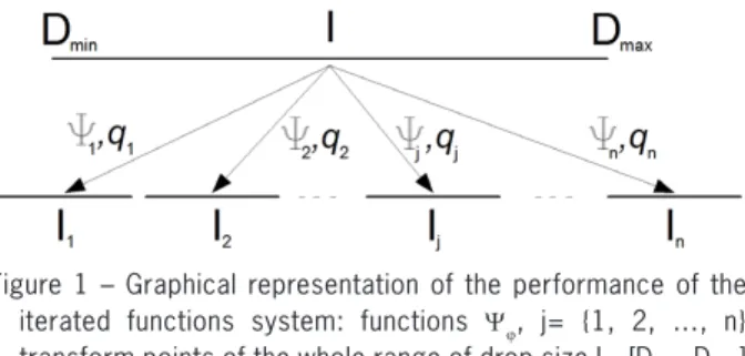
Secondly, Df was estimated as follows: let I1= [Dmin,
Dv1], I2= (Dv1, Dv2], …, Ij= (Dvj-1, Dvj], …, In= (Dvn-1, Dmax], which are the sub-intervals of the sizes corresponding
to the n droplet size spectra factor, where Dmin and Dmax
are the minimum and maximum droplet diameter, re-spectively. Thus, the whole range of droplet diameter
is I= [Dmin, Dmax]. In addition, q1, q2, …, qj, …, qn are the
relative volume proportions or probabilities (q1 + q2 +
…+ qj + …+ qn = 1) of volume intervals I1, I2, …, Ij, …,
In, respectively.
The following functions may be considered:
(
)
−Ψ = + − ×
− v1 min
1 min min
max min
D D
D D
D D
x
(
)
−Ψ = + − ×
−
v2 v1
2 v1 min
max min
D D
D D
D D
x
(
)
−Ψ = + − ×
− vj vj-1
j j-1 min
max min
D D
D D
D D
x
(
)
−Ψ = + − ×
− max vn-1
n n-1 min
max min
D D
D D
D D
x
where: x∈[Dmin, Dmax]. In the equations 5 to 8, Ψj, j=
{1, 2, …, n} are the linear functions that transform the
[Dmin, Dmax] points into Ij, j= {1, 2, …,n} points. The set
{Ψj; qj; j= {1, 2, …,n}} is called an ‘iterated function
(5)
(6)
(7)
system’ (Barnsley and Demko, 1985). By means of the
similarities Ψj and the volume proportions qj, an
iter-ated function system determines how a fractal distribu-tion reproduces its structure at different scales. Figure 1 shows a graphical representation of the performance of
the iterated functions system: each function Ψj, with j=
{1, 2, …,n} transforms values of the whole range of drop
diameters [Dmin, Dmax] into points of the ranges Ij, with j=
{1, 2, …,n}. For example, function Ψ1 transform the
val-ues of [Dmin, Dmax] into values of I1, taking into account
equation (1), and so for the rest of Ψjs. Furthermore, the
probability of use the function Ψj is qj, which is the
vol-ume fraction accumulated in the range Ij.
This second method to estimate the fractal dimen-sion has been developed because usually, data supplied by the nozzle manufacturer is the volumetric droplet size
distribution. So, available data are Dv’s instead of cloud
droplet diameters. Using fractal geometry, an algorithm
can be defined to obtain Df of a nozzle (Elton, 1987;
Tur-cotte, 1992): i) take any value x0 of [Dmin, Dmax]; ii)take
a random number j, j= {1, 2, …, n}, being qj= {q1, q2,
…, qn} their respective probabilities, and compute x1=
Ψj(x0); and iii) repeat step 2 taking x1 to compute the next
value. In this way, a set S= {x1, x2, ..., xm} is obtained.
This is not a set of droplets, instead these elements allow us to obtain the droplet diameter versus the cumu-lative volume fraction function and from this function we can then obtain the droplet size distribution, as
fol-lows: if g is the number of x’s values that belong to any
interval Ij, the ratio g/m approaches the relative volume
of the interval Ij as the number of iterations m goes to
infinite. For example, if droplet size spectra factors
mea-surements were Dv0.1= 147, Dv0.5= 464, and Dv0.9= 1000
µm and the elements generated by the algorithm
cor-responding to this test {x1, x2,…, xm} are sorted by ‘size’,
there will be 0.1 × m elements with a size equal or less
than 147 (Dv0.1); 0.5 × m elements with a size equal or
less than 464 (Dv0.5); and 0.9 × m elements with a size
equal or less than 1000 (Dv0.9).
Df of this set will be computed taking into account
equation (2), which can be particularized as follows
Nx < X = k× Xd (9)
where k is a constant. It can be rewritten as
log (Nx < X) = log(k) + d× log(X) (10)
Therefore, Df = 3-d will be derived from the
re-gression coefficient of the linear rere-gression fitted
be-tween log(Nx<X) and log(X).
The number m of elements generated in each ap-plication of this algorithm were 10000, and the initial
value for x (x0) was Dv0.9. Similar results could be
ex-pected if m ≥ 3000 and x0 takes any value of [Dmin, Dmax]
(Taguas et al., 1999).
A total of ten iterated function systems differing in number and combination of droplet size spectra factors
(Table 1) were used to estimate Df (Dfe) in order to study
the accuracy of the algorithm described when applied to each of these combinations. Fractal dimension was also estimated in two ways: 1) by taking into account
all operating pressures (Dfe); and 2) by taking into
ac-count only the extreme operating pressure of 2 and 10 bar (Dfe1).
The size frequency distribution of every set Sq=
{x1, x2, ..., xm } was calculated by dividing the size range
into 20 classes (Steel and Torrie, 1980). The number of elements in each class was counted and the linear
re-gression between log(N > x) and log(x) was carried out
using the droplet size spectra factors corresponding to
Figure 1 – Graphical representation of the performance of the iterated functions system: functions Ψj, j= {1, 2, …, n} transform points of the whole range of drop size I= [Dmin, Dmax] into points of the ranges Ij, j= {1, 2, …,n}. The probability of use a function Ψj is qj.
Table 1 – Droplet size spectra factor combinations taken into account when applying the algorithm based on the iterated function system. A cross indicates that the value concerned has been considered. In the first row,Dvx indicate droplet size spectra factors corresponding with x%.
Combination Dv0.05 Dv0.1 Dv0.15 Dv0.2 Dv0.25 Dv0.3 Dv0.35 Dv0.4 Dv0.45 Dv0.5 Dv0.55 Dv0.6 Dv0.65 Dv0.7 Dv0.75 Dv0.8 Dv0.85 Dv0.9 Dv0.95 Dv1
1 X X X X X X X X X X X X X X X X X X X X
2 X X X
3 X X X X X
4 X X X X X
5 X X X X X X X
6 X X X X X X X
7 X X X X X X X
8 X X X X X X X X X
9 X X X X X X X X X X X
extreme operating pressures (2 and 10 bar). This task was carried out by a computer program developed by the authors using Visual Basic 6.0.
Droplet size spectra factors were predicted using an exponential function as follows:
Dvh = exp(a + b × p + c × Dfe1) (11)
where: Dvh can be Dv0.1, Dv0.5 or Dv0.9 (µm) of a given
noz-zle, p is the operating pressure (bar), and Dfe1 is the
frac-tal dimension, estimated as described above (‘A fracfrac-tal approach to droplet size distribution’ section). The data used to carry out this regression were those from operat-ing pressures of 0.4, 0.6 and 0.8 Mpa, which were not
used to estimate Dfe1.
Results and Discussion
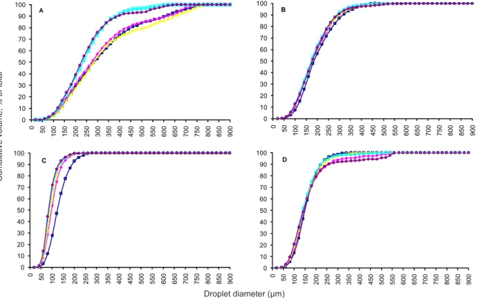
For a given nozzle, differences between functions representing each operating pressure presented no effect (Figure 2). Nevertheless, the DG-110 (Figure 2a) behav-ior at 0.8 and 1 MPa was very similar, and was quite dif-ferent from its behavior at other pressures. Furthermore, the TXA-80 nozzle (Figure 2c), shows differences with different operating pressures. In general, a higher spray pressure corresponded to a smaller droplet size spec-trum. These results are similar to those found by Womac (2001) working with nozzles under a range of pressures.
Furthermore, when the nozzles were compared, the cumulative volumetric droplet size distributions were quite different. All these affirmations about the cumula-tive droplet size distribution are based on an ANOVA
carried out comparing Dv10, Dv25, Dv50, Dv75 and Dv90 of
each nozzle working at 0.2, 0.4, 0.6, 0.8 and 1 MPa (data not presented). Similarity cumulative volumetric droplet size distribution behavior was related with nozzle type: TP-9501 and XR-110 are flat fan nozzles whereas DG-110 is a drift guard flat fan and TXA-80 is a hollow cone nozzle. Droplet sizes vary from a few micrometers up to some hundreds of micrometers depending on the nozzle type. Cone nozzle (TXA-80), produced the finest droplet size spectrum, followed by flat fan nozzles (TP-9501 and XR-110) and drift guard nozzle (DG-110). Nuyttens et al. (2007) observed the same behavior for these kinds of nozzles under a range of pressures.
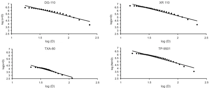
Fractal dimension, calculated taking into account
equation (1), can be considered the ‘real Df’ given that it
is derived from the droplet diameter measurements from each experiment. Figure 3 shows an example of
relation-ship between log(D) and log(Nd>D), and the fitted line
for each tested nozzle. To clarify these graphics, only 10 % approximately of data of each nozzle have been plot-ted. Anyway, the regressions have taken into account the whole data set. Although data had not a perfect straight tendency, which means no perfect fractal behavior, all studied cases (nozzle, operation pressure and
replica-0 10 20 30 40 50 60 70 80 90 100
0 50
100 150 200 250 300 350 400 450 500 550 600 650 700 750 800 850 900
A
0 10 20 30 40 50 60 70 80 90 100
0
50 100 150 200 250 300 350 400 450 500 550 600 650 700 750 800 850 900 B
0 10 20 30 40 50 60 70 80 90 100
0 50
100 150 200 250 300 350 400 450 500 550 600 650 700 750 800 850 900 C
0 10 20 30 40 50 60 70 80 90 100
0 50
100 150 200 250 300 350 400 450 500 550 600 650 700 750 800 850 900 D
Cumulative volume, % of total
Droplet diameter (µm)
tion) shown similar behavior: the relationship between
variables was correlated (p < 0.01). Furthermore, all
re-gression coefficients indicate that the model as fitted ex-plained more than 90 % of the variability in dependent variable (log(Nd>D)).
Table 2 shows the average ‘real fractal dimen-sion’ for each nozzle, operating pressure and repetitions studied, which have been calculated taking into account
measured droplet diameters. The Dfr column shows the
Df average calculated based on the values
correspond-ing to the five operatcorrespond-ing pressures, while the Dfr column
shows the Df average calculated from the extreme
pres-sures (0.2 and 1 MPa). Since Df is not a measurable
phys-ical magnitude, we have decided to report these values to an accuracy of four decimal places, although we have not looked at the effect of decimal places on our results.
Values shown in each row are different (p < 0.05),
whereas the values shown in each column are not
differ-ent (p > 0.05) (Table 2). Thus, the Df calculated in this
way and associated with nozzles, results in values which are independent of operating pressure. Similar results were found by Agüera et al. (2006) when working with hydraulic nozzles with variable geometry.
Table 3 shows the Dfe for every nozzle and Dv
com-bination (Table 1) when the algorithm based on iterated function systems described as the second method in ‘Calculating the fractal dimension’ section was applied. The column labeled ‘sd’ indicates the standard
devia-tion of Dfe derived from the five operating pressures and
the three repetitions, whereas r2
max and r
2
min indicate
the maximum and minimum regression coefficients of
linear regression between log(Nx<X) and log(X). Column
Dfe1 represents the fractal dimension for every nozzle,
considering data from operating pressures of 0.2 and 1
MPa, and Dv combinations when the algorithm based
on iterated function was applied. For a given nozzle and
column, Dfe or Dfe1 values followed by the same letter
are not different (p < 0.05). Dfeand Dfe1 estimated taking
into account Dv combination 1 can be regarded as being
the nearest to the ‘real Df’ shown in Table 2, given that
the 20 Dv values were used with the iterate function
sys-tem. In fact, the values shown in columns Dfr or Dfr1 of
Table 2 are not different (p < 0.05) from those of Table
3 corresponding to combination 1. Relationship between log(Nx<X) and log(X) were correlated (p < 0.01). Further-more, all regression coefficients indicate that the model as fitted explained the variability in dependent variable
(log(Nd>D)) between 0.826 (observed in the TXA-80
noz-zle) and 0.979 (observed in the DG-110 noznoz-zle).
Dv combination numbers 2, 4 and 5 yielded Dfe
values which were different from those of the
remain-ing Dv combinations. Combination 2 includes only three
Dv values: Dv0.1, Dv0.5 and Dv0.9, which are probably not
2.5 3 3.5 4 4.5 5 5.5 6 6.5 7
1 1.5 2 2.5
log (x>D)
2.5 3 3.5 4 4.5 5 5.5 6 6.5 7
1 1.5 2 2.5
log(x>D)
2.5 3 3.5 4 4.5 5 5.5 6 6.5 7
1 1.5 2 2.5
log(x>D)
2.5 3 3.5 4 4.5 5 5.5 6 6.5 7
1 1.5 2 2.5
log (Nd>D)
DG-110
TXA-80 TP-9501
XR 110
log (D)
log (D)
log (D)
log (D)
Figure 3 – Examples of relationship between log(D) and log(Nd>D), and the fitted line for each tested nozzle. For DG-110 nozzle: log(Nd>D)= 9.40 - 2.13 × log(D), r2= 0.93), operating pressure: 0.8 MPa; for XR-110 nozzle: log(N
d>D)= 9.70 - 2.24 × log(D), r
2= 0.95), operating pressure: 0.2 MPa; for TXA-80
nozzle: log(Nd>D)= 7.87 - 2.50 × log(D), r2= 0.95), operating pressure: 0.8 MPa; for TXA-80 nozzle: log(N
d>D)= 9.36 - 2.32 × log(D), r
2= 0.93), operating
pressure: 0.4 MPa. D is the droplet diameter (µm) and Nd>D is the cumulative number of size d droplets greater than a characteristic diameter.
Table 2 – Df (fractal dimension) for each nozzle and each pressure, calculated from droplets population, taking into account eq. (1). Dfr is the fractal dimension calculated as the average of fractal dimensions from the five operating pressures and Dfr1 is the fractal dimension calculated as the average of fractal dimensions from extreme operating pressures (0.2 and 1 MPa).
Df
Operating pressure (bar)
nozzle 2 4 6 8 10 Dfr Dfr1
enough to obtain precise Df values. Combination 4
adds two values of Dv: Dv0.15 and Dv0.85, with respect to
combination 2, while combination 5 adds four values
with respect to combination 2: Dv0.15, Dv0.25, Dv0.75 and
Dv0.85. All these values are between Dv0.1 and Dv0.9, situ-ated in the constant-slope zone of the curve diameter vs. cumulative volume. Similar results were obtained
for combination 3 which includes Dv values in these
areas, or combinations which include values between Dv0.25 and Dv0.75, except combination 1. Nevertheless, a
combination including Dv0.1, Dv0.5, Dv0.9 and other values
around Dv0.1 and Dv0.9 (combinations 7 and 10) yielded
the Dfe values nearest to that yielded by combination 1.
In Table 3, combinations 1, 7 and 10 are those which are included only in group ‘a’.
Dv combinations are not as influential in the
esti-mated fractal dimension as in the Dfe column: the Dfe1
value for the XR-110 and TP-9501 nozzles was
indepen-dent of Dv combinations, while the Dfe1 value for the
DG-110 and TXA-80 nozzles does not show differences
with the Dfe values (Table 3). Using iterated function
systems and several combinations of soil particles size spectra factors to simulate and to test of self-similar structures for soil-size distributions, Taguas et al. (1999) found relationship between the used combination and the results accuracy.
As the Dfe values from Dv combination 10 are the
nearest to those from Dv combination 1, except for the
TXA-80 nozzle, Dfe1 values from Dv combination 10 were
used to fit data in equation (11). Coefficients of deter-mination and regression coefficients as determined by regression modeling of droplet size factors were:
Dv0.1=exp (11.0534 – 0.01877 × p – 2.82532 × Dfe1); r2 = 0.8931(12)
Dv0.5=exp(14.0725 – 0.02102 × p – 3.89492 × Dfe1); r2=0.8783 (13)
Dv0.9=exp(16.9797 – 0.04216 × p – 4.87581 × Dfe1); r2 =0.8447(14)
where: Dfe1 is the own fractal dimension value of each
nozzle shown in Table 3 for combination 10, Dv0.1, Dv0.5 or
Dv0.9 are µm) and p is the operating pressure (0.1×MPa).
Coefficients of determination which were
signifi-cant (p < 0.05) tended to have decreasing r2 values with
increasing droplet size factors, which is a similar behav-ior to that observed by Agüera et al. (2006) using poly-nomial and multilinear fitted regressions and also to that observed by Womac (2001) using a multilinear fitted re-gression, although in both these studies the authors found some non-significant coefficients of determination.
Conclusions
The algorithm resulted in Df values similar to
those calculated from measured droplet diameter (‘real
Df’), regardless of the operating pressure and related to
the nozzle type. Df for a given nozzle can be calculated
from two droplet size spectra measurements performed
Table 3 – Estimated Df (fractal dimension) for every nozzle and Dv (droplet size spectra factors) combinations when the algorithm based on iterated function was applied. The sd column indicates the standard deviation of Dfe (fractal dimension derived from the five operating pressures and the three repetitions). Columns r2
max and r 2
min indicate the maximum and minimum coefficients
of determination of linear regression between log(Nx<X) (being Nx>X the cumulative number of diameter x droplets greater than a characteristic average diameter X of a sub-set containing 500 droplets) and log(X) (being X the average diameter of a sub-set containing 500 droplet), respectively. Column Dfe1 represents fractal dimension for every nozzle, taking into account data from operating pressure of 0.2 and 1 MPa, and Dv (droplet size spectra factors) combinations when the algorithm based on iterated function was applied. For a given nozzle and column, Dfe or Dfe1 values followed by the same letter are not different (p < 0.05).
nozzle Dv
combination Dfe sd r
2
min r
2
max Dfe1
DG-110 1 2.2005a 0.0558 0.899 0.970 2.1842a
DG-110 2 2.0782b 0.0809 0.906 0.975 2.0488b
DG-110 3 2.2079a 0.0676 0.890 0.967 2.1868a
DG-110 4 2.0726b 0.0744 0.909 0.975 2.0553b
DG-110 5 2.0815b 0.0738 0.915 0.979 2.0650b
DG-110 6 2.2022a 0.0581 0.884 0.963 2.1792a
DG-110 7 2.2047a 0.0560 0.884 0.967 2.1951a
DG-110 8 2.2006a 0.0563 0.888 0.969 2.1798a
DG-110 9 2.1974a 0.0541 0.888 0.967 2.1845a
DG-110 10 2.2006a 0.0559 0.880 0.972 2.1788a
XR-110 1 2.2439a 0.0865 0.864 0.977 2.2695a
XR-110 2 2.1137c 0.1248 0.860 0.973 2.1526a
XR-110 3 2.2398a,b 0.0837 0.826 0.975 2.2591a
XR-110 4 2.1264b,c 0.1250 0.861 0.977 2.1709a
XR-110 5 2.1240c 0.1173 0.875 0.977 2.1547a
XR-110 6 2.2426a 0.0938 0.846 0.976 2.2652a
XR-110 7 2.2413a 0.0823 0.836 0.977 2.2644a
XR-110 8 2.2405a,b 0.0865 0.858 0.976 2.2631a
XR-110 9 2.2400a,b 0.0841 0.861 0.978 2.2659a
XR-110 10 2.2439a 0.0846 0.844 0.977 2.2670a
TXA-80 1 2.4440a 0.0270 0.935 0.972 2.4424a
TXA-80 2 2.3322b 0.0422 0.941 0.967 2.3237b
TXA-80 3 2.4455a 0.0265 0.930 0.974 2.4437a
TXA-80 4 2.3274b 0.0354 0.940 0.970 2.3208b
TXA-80 5 2.3263b 0.0376 0.940 0.972 2.3215b
TXA-80 6 2.4438a 0.0282 0.938 0.975 2.4461a
TXA-80 7 2.4465a 0.0250 0.934 0.970 2.4387a
TXA-80 8 2.4473a 0.0222 0.937 0.975 2.4393a
TXA-80 9 2.4425a 0.0269 0.934 0.973 2.4394a
TXA-80 10 2.4401a 0.0233 0.937 0.972 2.4340a
TP-9501 1 2.2209a 0.1077 0.862 0.968 2.2593a
TP-9501 2 2.0661d 0.1325 0.831 0.959 2.1095a
TP-9501 3 2.2155a 0.1095 0.843 0.964 2.2469a
TP-9501 4 2.0718c,d 0.1416 0.841 0.964 2.1173a
TP-9501 5 2.0761b,c,d0.1361 0.859 0.965 2.1004a
TP-9501 6 2.2119a,b 0.1136 0.862 0.967 2.2494a
TP-9501 7 2.2176a 0.1059 0.844 0.968 2.2494a
TP-9501 8 2.2161a 0.1117 0.867 0.968 2.2554a
TP-9501 9 2.2084a,b,c0.1082 0.866 0.968 2.2429a
at extreme operating pressure (0.2 and 1 MPa), thus eliminating the need for droplet size measurements at
intermediate operating pressures. Dv0.1, Dv0.5 and Dv0.9
for the nozzles tested at 0.2 and 1 MPa pressure can be estimated at any operating pressure from this exponen-tial model.
Acknowledgements
This work was supported by grant P07-AGR-02995 from CICE - Junta de Andalucia (Spain), co-financed with FEDER funds of the European Union.
References
Agüera, F.; Aguilar, F.J.; Aguilar, M.A.; Carvajal, F. 2006. Atomization characteristics of hydraulic nozzles using fractal geometry. Transaction of the ASABE 49: 581–587.
ASAE Standards. 1997. S327.2: Terminology and definitions for agricultural chemical applications. ASAE Standards. 44th ed. St. Joseph, Mich.: ASAE.
Baetens, K.; Nuyttens, D.; Verboven, P.; De Schampheleire, M.; Nicolaï, B.; Ramon, H. 2007. Predicting drift from field spraying by means of a 3D computational fluid dynamics model. Computers and Electronics in Agriculture. 56: 161–173. Baetens, K.; Ho, Q. T.; Nuyttens, D.; De Schampheleire, M.; Melese
Endalew, M.; Hertog, M.; Nicolaï, B.; Ramon, H; Verboven, P. 2009. A Validated 2-D diffusion-advection model for prediction of drift from ground boom sprayers. Atmospheric Environment 43: 1674–1682.
Eghball, B.; Mielke, N.M.; Calvo, G.A.; Wilhelm, W.W. 1993. Fractal description of soil fragmentation for various tillage methods and crop sequences. Soil Science Society of America Journal 57: 1337–1341.
Elton, J. 1987. An ergodic theorem for iterated maps. Journal of Ergodic Theory and Dynamical Systems 7: 481–488.
Mandelbrot, B.B. 1982. The fractal geometry of nature. W.H. Freeman, New York, NY, USA.
Nuyttens, D.; Baetens, K.; De Schampheleire, M.; Sonck, B. 2007. Effect of nozzle type, size and pressure on spray droplet characteristics. Biosystems Engineering 97: 333–345.
Nuyttens, D.; De Schampheleire, M.; Verboven, P.; Sonck, B. 2010. Comparison between indirect and direct spray drift assessment methods. Biosystems Engineering. 105: 2–12.
Nuyttens, D.; De Schampheleire, M.; Baetens, K.; Brusselman, E.; Dekeyser, D.; Verboven, P. 2011. Drift from field crop sprayers using an integrated approach: results of a 5 year study. Transactions of the ASABE 54: 403–408
Perfect, E.; Bird, N.; Rieu, M. 1992. Generalizing the fractal model of soil structure: the pore-solid fractal approach. Geoderma 88: 137–164.
Steel, R.G.D; Torrie, J.H. 1980. Principles and Procedures of Statistics: biometrial approach. McGraw-Hill, New York, NY, USA.
Taguas, F.J.; Martín, M.A.; Perfect, E. 1999. Simulation and testing of self-similar structures, for soil particle-size distributions using iterated function systems. Geoderma 88: 191–203. Turcotte, D.L. 1992. Fractals and Chaos in Geology and
Geophysics. Cambridge University Press, Cambridge, UK. Tyler, S.W.; Wheatcraft, S.W. 1992. Fractal scaling for soil
particle-size distributions: analysis and limitations. Soil Science Society of America Journal 56: 362–369.
Teske, M.E.; Thistle, H.W.; Mickle, R.E. 2000. Modeling finer droplet aerial spray drift and deposition. Applied Engineering in Agriculture 16: 351–357.
Womac, A.R. 1999. Measurements variations in reference sprays for nozzle classification. Transaction of ASAE 42: 609–616. Womac, A.R. 2001. Atomization characteristics of high-flow
variable-orifice flooding nozzles. Transaction of ASAE 44: 463–471. Zhu, H.; Reichard, D.L.; Fox, R.D.; Brazee, R.D.; Ozkam, H.E.