www.atmos-chem-phys.net/9/2891/2009/ © Author(s) 2009. This work is distributed under the Creative Commons Attribution 3.0 License.
Chemistry
and Physics
Interpretation of organic components from Positive Matrix
Factorization of aerosol mass spectrometric data
I. M. Ulbrich1,2, M. R. Canagaratna3, Q. Zhang4, D. R. Worsnop3, and J. L. Jimenez1,2
1Cooperative Institute for Research in the Environmental Sciences (CIRES), Boulder, CO, USA 2Department of Chemistry and Biochemistry, University of Colorado, Boulder, CO, USA 3Aerodyne Research, Inc., Billerica, MA, USA
4Atmos. Sci. Res. Center, University at Albany, State University of New York, Albany, NY, USA
Received: 27 February 2008 – Published in Atmos. Chem. Phys. Discuss.: 9 April 2008 Revised: 2 April 2009 – Accepted: 14 April 2009 – Published: 5 May 2009
Abstract. The organic aerosol (OA) dataset from an Aero-dyne Aerosol Mass Spectrometer (Q-AMS) collected at the Pittsburgh Air Quality Study (PAQS) in September 2002 was analyzed with Positive Matrix Factorization (PMF). Three components – hydrocarbon-like organic aerosol OA (HOA), a highly-oxygenated OA (OOA-1) that correlates well with sulfate, and a less-oxygenated, semi-volatile OA (OOA-2) that correlates well with nitrate and chloride – are identified and interpreted as primary combustion emissions, aged SOA, and semivolatile, less aged SOA, respectively. The complex-ity of interpreting the PMF solutions of unit mass resolution (UMR) AMS data is illustrated by a detailed analysis of the solutions as a function of number of components and rota-tional forcing. A public web-based database of AMS spectra has been created to aid this type of analysis. Realistic syn-thetic data is also used to characterize the behavior of PMF for choosing the best number of factors, and evaluating the rotations of non-unique solutions. The ambient and synthetic data indicate that the variation of the PMF quality of fit pa-rameter (Q, a normalized chi-squared metric) vs. number of factors in the solution is useful to identify the minimum number of factors, but more detailed analysis and interpre-tation are needed to choose the best number of factors. The maximum value of the rotational matrix is not useful for de-termining the best number of factors. In synthetic datasets, factors are “split” into two or more components when solv-ing for more factors than were used in the input. Elements of the “splitting” behavior are observed in solutions of real datasets with several factors. Significant structure remains in the residual of the real dataset after physically-meaningful factors have been assigned and an unrealistic number of
fac-Correspondence to:J. L Jimenez (jose.jimenez@colorado.edu)
tors would be required to explain the remaining variance. This residual structure appears to be due to variability in the spectra of the components (especially OOA-2 in this case), which is likely to be a key limit of the retrievability of com-ponents from AMS datasets using PMF and similar meth-ods that need to assume constant component mass spectra. Methods for characterizing and dealing with this variabil-ity are needed. Interpretation of PMF factors must be done carefully. Synthetic data indicate that PMF internal diagnos-tics and similarity to available source component spectra to-gether are not sufficient for identifying factors. It is critical to use correlations between factor and external measurement time series and other criteria to support factor interpretations. True components with<5% of the mass are unlikely to be retrieved accurately. Results from this study may be useful for interpreting the PMF analysis of data from other aerosol mass spectrometers. Researchers are urged to analyze future datasets carefully, including synthetic analyses, and to evalu-ate whether the conclusions made here apply to their datasets.
1 Introduction
The organic source apportionment problem has been approached by several techniques. Turpin and Huntz-icker (1991) utilized the ratio between elemental carbon and organic carbon (EC/OC) from filter samples to estimate pri-mary and secondary OA. Schauer et al. (1996) used molecu-lar markers with a chemical mass balance (CMB) approach to apportion OA extracted from filters and analyzed by GC-MS. Several sources with unique markers can be identified, but source profiles must be known a priori, sources without unique markers are not easily separated, and only primary OA sources are identified. Szidat et al. (2006) have sepa-rated anthropogenic and biogenic OA based on water solubil-ity and14C/12C ratios and found a major biogenic influence in Zurich, Switzerland. The technique has very low time res-olution (many hours to several days) and can identify only a few categories of sources. Traditional OA filter measure-ments suffer from low time resolution (several hrs. to days) and positive and negative artifacts (Turpin et al., 2000).
The last 15 years have seen the development of a new gen-eration of real-time aerosol chemical instrumentation, most commonly based on mass spectrometry or ion chromatogra-phy (Sullivan et al., 2004; DeCarlo et al., 2006; Williams et al., 2006; Canagaratna et al., 2007; Murphy, 2007). Cur-rent real-time instruments can produce data over timescales of seconds to minutes and have reduced sampling artifacts compared to filters. Single-particle mass spectrometers (e.g., PALMS, ATOFMS, SPLAT) have used particle classification systems to group particles based on composition or other characteristics (Murphy et al., 2003). A fast GC-MS sys-tem (TAG) has been developed that may allow the applica-tion of the molecular marker technique with much faster time resolution than previously possible (Williams et al., 2006). However GC-MS as typically applied discriminates against oxygenated organic aerosols (OOA) (Huffman et al., 2009), which is the dominant ambient OA component (Zhang et al., 2007a), and thus may limit the applicability of this technique by itself. It is highly desirable to perform source apportion-ment based on the composition of the whole OA. This infor-mation cannot be obtained at the molecular level with current techniques, however several techniques are starting to char-acterize the types/groups of species in bulk OA (Fuzzi et al., 2001; Russell, 2003; Zhang et al., 2005a, c).
The Aerodyne Aerosol Mass Spectrometer (AMS) be-longs to the category of instruments that seeks to measure and characterize the whole OA. It has been designed to quan-titatively measure the non-refractory components of submi-cron aerosol with high time resolution (Jayne et al., 2000; Jimenez et al., 2003) and produces ensemble average spectra for organic species every few seconds to minutes (Allan et al., 2004). Several groups have attempted different methods to deconvolve the OA spectral matrix measured by a Q-AMS (Zhang et al., 2005a, c, 2007a; Marcolli et al., 2006; Lanz et al., 2007). Zhang et al. (2005a) first showed that information on OA sources could be extracted from linear decomposition of AMS spectra by using a custom principal component
anal-ysis (CPCA) method applied to OA data from the Pittsburgh Supersite from 2002. The resulting factors were identified as hydrocarbon-like organic aerosol (HOA, a reduced OA) and oxygenated organic aerosol (OOA) and were strongly linked to primary and secondary organic aerosol (POA and SOA), respectively, based on comparison of their spectra to known sources and their time series to other tracers. OOA was found to dominate OA (∼2/3 of the OA mass was OOA), in con-trast to previous results at this location (Cabada et al., 2004). Zhang et al. (2007a) used the Multiple Component Analy-sis technique (MCA, an expanded version of the CPCA) for separating more than two factors in datasets from 37 field campaigns in the Northern Hemisphere and found that the sum of several OOAs comprises more of the organic aerosol mass than HOA at most locations and times, and that in rural areas the fraction of HOA is usually very small. Marcolli et al. (2006) applied a hierarchical cluster analysis to Q-AMS data from the New England Air Quality Study (NEAQS) from 2002. Clusters in this data represented biogenic VOC oxidation products, highly oxidized OA, and other small cat-egories. Lanz et al. (2007) applied Positive Matrix Factor-ization (PMF) (Paatero and Tapper, 1994; Paatero, 1997) to the organic fraction of a Q-AMS dataset from Zurich in the summer of 2005. The six factors identified in this study were HOA, two types of OOA (a highly-oxidized, thermody-namically stable type called OOA-1 that correlates well with aerosol sulfate; and a less-oxidized, semi-volatile type called OOA-2 that correlates well with aerosol nitrate), charbroil-ing, wood burncharbroil-ing, and a minor source that may be influ-enced by food cooking. Lanz et al. (2008) applied a hybrid receptor model (combining CMB-style a priori information of factor profiles with the bilinear PMF model) specified by the Mulilinear Engine (ME-2, Paatero, 1999) to apportion the organic fraction of a Q-AMS dataset from Zurich during win-tertime inversions, when no physically-meaningful compo-nents could be identified by the bilinear model alone. Three factors, representing HOA, OOA, and wood burning aerosol, were identified, with OOA and wood-burning aerosol ac-counting for 55% and 38% of the mass, respectively. More advanced source apportionment methods based on Bayesian statistics, which output a probability distribution instead of scalars for each element of the source profiles and time se-ries and thus contain information necessary for a statistical evaluation of the uncertainty of the output, are under de-velopment (Christensen et al., 2007; Lingwall et al., 2008). Bayesian models can also incorporate prior information in a natural and probabilistically rigorous way by specification of the “prior distribution” for each variable. Bayesian methods are expensive computationally, and the more complex output requires greater review by the researcher. Bayesian methods have not been applied to aerosol MS data to our knowledge.
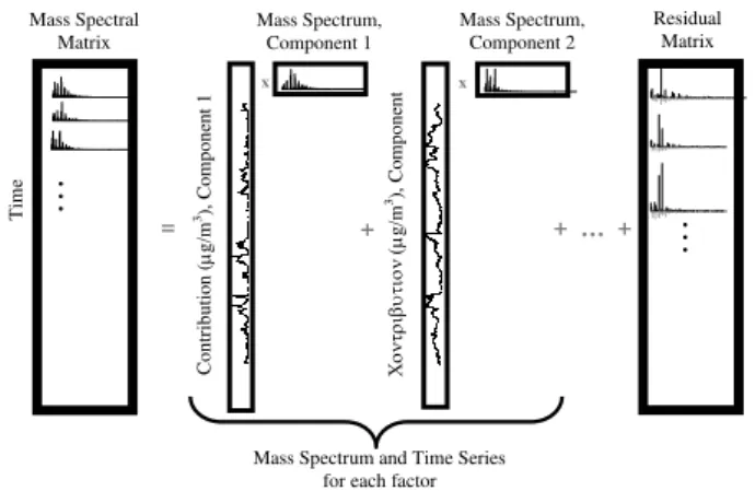
2003) and its application to PM has been recently summa-rized in two separate reviews (Reff et al., 2007; Engel-Cox and Weber, 2007). PMF is a receptor-only, factorization model based on mass conservation which requires no a pri-ori information about factor profiles or time trends. PMF has generally been applied to long-term, low-time-resolution datasets, though there has been a call for greater application of source apportionment techniques to air pollution events to facilitate understanding of specific sources for regulatory purposes (Engel-Cox and Weber, 2007). As shown schemat-ically in Fig. 1, PMF is a bilinear unmixing model in which a dataset matrix is assumed to be comprised of the linear com-bination of factors with constant profiles that have varying contributions across the dataset. All of the values in the pro-files and contributions are constrained to be positive. The model can have an arbitrary number of factors; the user must select the solution that “best” explains the data. This is often the most subjective and least quantitative step of PMF anal-ysis and relies greatly on the judgment and skill of the mod-eler (Engel-Cox and Weber, 2007; Reff et al., 2007). In ad-dition, mathematical deconvolution of a dataset often yields non-unique solutions, in which linear transformations (collo-quially referred to as “rotations”) of the factors are possible while the positivity constraint is maintained. The necessity of choosing a number of factors and a particular rotation of-ten complicates the interpretation of the solutions. As clearly articulated by P. Paatero, personal communication, 2007:
“It is unfortunate that introducing a priori information also introduces some subjectivity in the analysis [. . . ] However, the tradeoff is often between a successful albeit subjectively aided analysis and an unsuccessful analysis. [. . . ] subjective decisions must be fully and openly reported in publications. [. . . ] Hiding the details of subjective decisions or even worse, pretending that no subjectivity is included in the analysis, should not be tolerated in scientific publications”.
Although the application of PMF analysis to data from the AMS and other aerosol mass spectrometers is relatively new, it is quickly becoming widespread. Thus, a detailed charac-terization of the capabilities and pitfalls of this type of anal-ysis when applied to aerosol MS data is important. UMR AMS datasets are very large with typically several million datapoints (∼300m/z’s per sample, with∼8000 samples for a month-long campaign with 5 min averaging) and fragmen-tation of molecules during ionization gives each mass spec-trum strongly interrelated data. AMS datasets differ in two fundamental ways from most atmospheric datasets to which PMF has been applied. The structure, internal correlation between somem/z’s created by significant fragmentation of molecules in the vaporization and ionization processes in the AMS, and precision of AMS data are significantly differ-ent from datasets of multiple aerosol compondiffer-ents (metals, organic and elemental carbon, ions, etc.) measured by sev-eral instruments typically used with PMF in previous studies. The error structure is also more coherent and self-consistent due to the use of data from a single instrument, rather than
= +
x
Contribution
(
µ
g/m
3), Componen
t 1
Mass Spectrum, Component 1
x
Χ
ον
τρ
ιβ
υτ
ιο
ν
(µ
g/m
3), Co
mpon
ent
Mass Spectrum, Component 2 Mass Spectral
Matrix
Time
+ … +
. . .
Residual Matrix
Mass Spectrum and Time Series for each factor
. . .
Fig. 1. Schematic of PMF factorization of an AMS dataset. The time series of the factors make up the matrixGand the mass spectra of the factors make up the matrixFin Eq. (1).
mixing data from different instruments for which the relative errors may be more difficult to quantify precisely, or that may drift differently, etc.
In this work, we apply PMF to data obtained with the quadrupole Aerosol Mass Spectrometer (Q-AMS) during the Pittsburgh Air Quality Study. Three factors, interpreted as HOA, aged regional OOA, and fresh, semivolatile OOA are reported for the Pittsburgh ambient dataset. The ambigui-ties associated with choosing the number of factors and their best rotations are reported. In addition, sensitivity analyses are performed with synthetic datasets constructed to retain the inherent structure of AMS data and errors. We explore methods that can inform the choice of the appropriate num-ber of factors and rotation for AMS OA datasets, as well as investigate the retrievability of small factors.
2 Methods
2.1 Aerosol Mass Spectrometer (AMS)
The Q-AMS can be operated in any of three modes: mass spectrum (MS), particle time-of-flight (PToF), or jump mass spectrum (JMS). In MS mode, the chopper alternates be-tween the beam open and closed positions while the mass spectrometer scans acrossm/z1 to 300. Each e.g. five-minute average is the difference between the total open and closed signals and is the ensemble average mass spectrum of thou-sands of particles. In PToF mode, the beam is chopped and packets of one or a few particles enter the particle sizing re-gion. Particles achieve size-dependent velocities at the exit of the lens which allows measurement of particle size dis-tributions, but only at∼10–15 selectedm/z’s. JMS mode is identical to MS mode except in that only∼10m/z’s are mon-itored to maximize signal-to-noise ratio (SNR) (Crosier et al., 2007; Nemitz et al., 2008). We use the MS mode data for this study because it has high signal-to-noise and con-tains the full structure of the mass spectra and thus the most chemical information. Each sample is the linear combina-tion of the spectra from all particles and species vaporized during the sample period. If JMS data is available, it may be used to replace the MSm/z’s as the JMS data has much better SNR (Crosier et al., 2007). Preliminary analyses show that PToF data contains significant information that can be ex-ploited by PMF-like methods (Nemitz et al., 2008), however this also introduces additional complexities and it is outside of the scope of this paper.
Newer versions of the AMS include the compact time-of-flight mass spectrometer (C-ToF-AMS, Drewnick et al., 2005) and the high-resolution ToF-AMS (HR-ToF-AMS, DeCarlo et al., 2006). These instruments operate in MS and PToF modes. Conceptually the MS mode from the C-ToF-AMS produces identical data to those from the Q-AMS, except with higher SNR, and thus the results from this pa-per should be applicable to PMF analyses of such data. The MS mode from the HR-ToF-AMS contains much additional chemical information such as time series of high resolution ions (e.g., both C3H+7 and C2H3O+instead of totalm/z43)
that facilitates the extraction of PMF components. The first application of PMF to HR-ToF-AMS MS-mode data has been presented in a separate publication (Aiken et al., 2009). The datasets used in this study are comprised of only the organic portion of the AMS mass spectrum measured by the Q-AMS, which is determined from the total mass spec-trum by application of a “fragmentation table” (Allan et al., 2004) for removing ions from air and inorganic species. The atomic oxygen to carbon ratio (O/C) for UMR MS can be estimated from the percent of OA signal atm/z44 (predom-inately CO+2)in the OA MS (Aiken et al., 2008). Percent
m/z44 is reported here as an indication of the degree of oxy-genation of representative spectra.
The time series of inorganic species (non-refractory am-monium, nitrate, sulfate, and chloride) are not included in the PMF analysis and are instead retained for a posteriori com-parison with the time series of the factors and for use in their interpretation. It is also of interest to perform the PMF
analy-sis on the total spectrum without removing inorganic species (but still removing the large air signals), however this is out-side the scope of this paper.
2.2 Factorization methods
2.2.1 Positive Matrix Factorization (PMF)
Positive Matrix Factorization (PMF) (Paatero and Tapper, 1994; Paatero, 1997) is a model for solving a receptor-only, bilinear unmixing model which assumes that a measured dataset conforms to a mass-balance of a number of con-stantsource profiles (mass spectra for AMS data) contribut-ing varycontribut-ing concentrations over the time of the dataset (time series), such that
xij =
X
p
gipfpj+eij (1)
wherei andj refer to row and column indices in the ma-trix, respectively,pis the number of factors in the solution, andxij is an element of themxnmatrixXof measured data
elements to be fit. In AMS data, themrows ofXare ensem-ble average mass spectra (MS) of typically tens of thousands of particles measured over each averaging period (typically 5 min) and then columns ofX are the time series (TS) of eachm/zsampled. gij is an element of themxpmatrix G whose columns are the factor TS,fij is an element of the
pxnmatrixFwhose rows are the factor profiles (MS), and
eij is an element of the mxn matrixE of residuals not fit by the model for each experimental data point (E=X−GF). A schematic representation of the factorization is shown in Fig. 1. The model requires no a priori information about the values of GandF. We normalize the rows in F (MS) to sum to 1, giving units of mass concentration (µg/m3)to the columns ofG(TS). The values ofGandFare iteratively fit to the data using a least-squares algorithm, minimizing a quality of fit parameterQ, defined as
Q=
m
X
i=1 n
X
j=1
(eij/σij)2 (2)
whereσij is an element of themxnmatrix of estimated
er-rors (standard deviations) of the points in the data matrix,X. In the “robust mode” of the algorithm, outliers (|eij/σij|>4)
are dynamically reweighted throughout the fitting process so that they cannot pull the fit with weight>4. TheQ-value reported by PMF is calculated using the reduced weights for the outliers. This scaling makes optimal use of the informa-tion content of the data by weighing variables by their de-gree of measurement certainty (Paatero and Tapper, 1994). It is possible that there may be multiple local minima of the
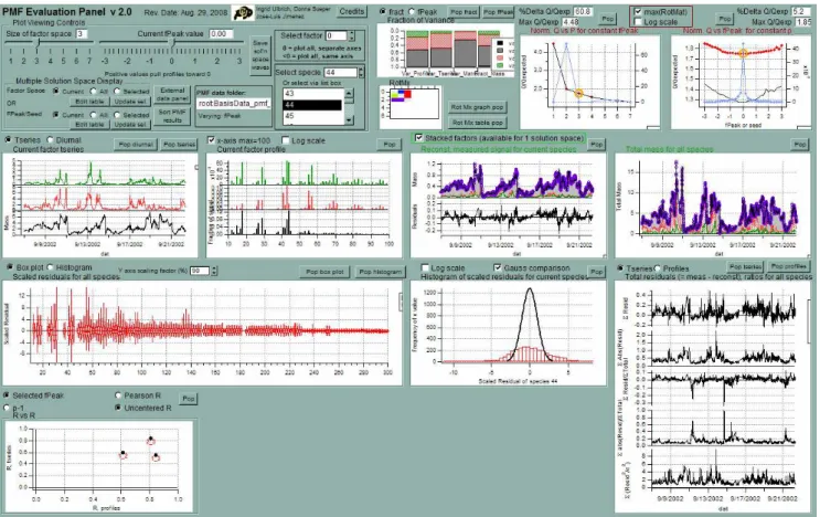
Fig. 2.Screenshot of PMF Evaluation Tool developed for general examination of PMF solutions.
be positive, reflecting positive contributions of each factor to the measured mass and positive signal in eachm/z, respec-tively.
The bilinear model can be solved by the PMF2 (Paatero, 2007) and multilinear engine (ME) (Paatero, 1999) algo-rithms developed by P. Paatero, or by custom algoalgo-rithms de-veloped by others (Lu and Wu, 2004; Lee and Seung, 1999; Hoyer, 2004). Here we use PMF2 because of its robustness and wide use in the research community. Future work will explore more complex models using the ME program. All analyses in this study were done with PMF2 version 4.2 in the robust mode, unless otherwise noted. The default conver-gence criteria were not modified. Since the output of PMF is very large and evaluating it is very complex, we developed a custom software tool (PMF Evaluation Tool, PET, Fig. 2) in Igor Pro (WaveMetrics, Inc., Portland, Oregon) to evaluate PMF outputs and related statistics. The PET calls the PMF2 algorithm to solve a given problem for a list of values ofp
and FPEAK or SEED, stores the results for all of these binations, and allows the user to rapidly display and com-pare many aspects of the solution matrix and residuals and to systematically evaluate the similarities and differences of the output spectra and time series with known source/component spectra and tracer time series.
Choosing the number of factors
The number of factors,p, in the real dataset is generally un-known. Choosing the best modeled number of factors for a dataset is the most critical decision to the interpretation of the PMF results. Several mathematical metrics have been used to aid determination of this value. A first criterion is theQ -value, the total sum of the squares of the scaled residuals. If all points in the matrix are fit to within their expected error, then abs (eij)/σij is∼1 and the expected Q(Qexp)equals
the degrees of freedom of the fitted data = mn−p(m+n)
(Paatero et al., 2002). For AMS datasets, mn≫p(m+n), so Qexp≈mn, the number of points in the data matrix. If
the assumptions of the bilinear model are appropriate for the problem (data is the sum of variable amounts of components with constant mass spectra) and the estimation of the errors in the input data is accurate, solutions with numbers of fac-tors that giveQ/Qexpnear 1 should be obtained. Values of Q/Qexp≫1 indicate underestimation of the errors or
variabil-ity in the factor profiles that cannot be simply modeled as the sum of the given number of components. IfQ/Qexp≪1, the
that should allow more of the data to be fit. A large decrease inQwith the addition of another factor implies that the addi-tional factor has explained significantly more of the variation in the data and has also been used as a metric for choosing a solution (Paatero and Tapper, 1993). A second metric for choosing a best solution is based on the values of the rota-tional matrix (RotMat, output by PMF and explained below). Some have used the criterion of a solution with the least ro-tation (lowest maximum value of Rotmat) as one of several qualitative metrics for making the determination of the num-ber of factors (Lee et al., 1999; Lanz et al., 2007). Many studies have concluded that source apportionment models must be combined with supplementary evidence to choose and identify factors (Engel-Cox and Weber, 2007).
Choosing the best number of factors requires the modeler to determine when additional factors fail to explain more of the variability in the dataset. Note that it is possible for one true factor to be mathematically represented by multiple fac-tors which, in total, represent the true factor (Paatero, 2008a). Consider a case in which two true factors make up the data with no error, such that
X=GF (3)
whereG=[ab], the matrix of the time series of the two fac-tors, andFT=[st]T, the matrix of the profiles of the two fac-tors, anda, b, s, andtare column vectors. If the same dataset Xis solved with three factors, an exact solution could be ob-tained as
X= [ef b] × [sst]T (4)
ife+f=a. In fact, a case could be constructed in which two factors reconstructb instead ofa, generating a second type of 3-factor solution. More combinations are possible when the sameXcreated with 2 factors is solved with 4 factors, e.g.,
X= [ef bb] × [ssuv]T (5)
wheree+f=aandu+v=t, or
X= [def b] × [ssst]T (6)
whered+e+f=a. We refer to this type of behavior as “split-ting” of the real factors, where either the MS or TS from a real factor are split into two new factors. Linear transfor-mations (“rotations”, discussed further in the next section) of these solutions are also possible. A rotation of the three-factor solution shown in Eq. (4) could be represented by
X= [ef b]T×T−1[sst]T (7)
whereT is a 3×3 non-singular transformation matrix and T−1is its inverse and is a valid solution to the PMF model as long as the rotated factor matrices [ef b]TandT−1[sst]T all have positive values. Thus the rotated solutions need not necessarily contain repetitions of the factors from the original solution (Paatero, 2008a). We refer to this later behavior as “mixing” of the real factors.
Rotational ambiguity of solutions
Despite the constraint of non-negativity, PMF solutions may not be unique, i.e., there may be linear transformations (“ro-tations”) of the factor time series and mass spectra that result in an identical fit to the data, such that:
GF=GTT−1F (8)
whereTis a transformation matrix andT−1is its inverse. A giventij>0 would create a rotation by adding the mass
spec-tra and subspec-tracting the time series of factorsi andj, while
tij<0 would create a rotation by subtracting the mass spectra and adding the time series of factorsiandj. An infinite num-ber of “rotations” may exist and still meet the non-negativity constraint. Note that orthogonal or “solid body” geometric rotations of the factors are only a subset of the possible lin-ear transformations.
PMF2 does not report the possible values ofT, but does report the standard deviation of possible values ofTas the “RotMat” matrix. Larger values inTimply greater rotational freedom of a solution. Specifically, a larger value oftij
sug-gests that theiandjfactors can be mixed in varying degrees while still satisfying the non-negativity constraint. Diagonal elements ofTare always 1, and their standard deviations are therefore 0. RotMat for a one-factor solution is always 0. The value of RotMat as a diagnostic has been debated in the literature (Lanz et al., 2007; Lee et al., 1999; Paatero, 2007), and we explore its use as a qualitative indicator of rotational freedom of a given solution (Sect. 3.1.2, 3.2.2).
With PMF2, once the approximate best number of factors has been determined, a subset of the rotational freedom of the solution may be explored through use of the FPEAK parame-ter. FPEAK allows for examining approximate or “distorted” rotations that do not strictly follow Eq. (7) and thus produce a higher value ofQ. Of greatest interest are FPEAK values for whichQdoes not increase significantly overQFPEAK=0,
since the PMF model (Eq. 2) is still satisfied with little addi-tional error. Some researchers recommend exploring a range of FPEAKs such thatQ/Qexp increases from its minimum
Uncertainty of the solutions
The difficult issue of the uncertainty of the solutions is rarely addressed in PMF studies in the literature (Reff et al., 2007). We address this point in this work in two ways: in a qualita-tive way by running the PMF algorithm from many different random starting points (SEEDs; Paatero, 2007), and quanti-tatively with bootstrapping with replacement of MS (Norris et al., 2008; Press et al., 2007a).
2.2.2 Singular value decomposition
In contrast to PMF, the singular value decomposition (SVD) of a matrix produces only one factorization (as in Eq. 1) with orthogonal factors. Starting with the factor that explains the most variance of the original matrix, factors are retained in order of decreasing variance of the matrix to explain enough (usually 99%) of the variance of the original matrix. These orthogonal factors usually contain negative values. SVD is applied to selected data matrices and residual matrices to de-termine the number of factors needed to explain 99% of the variance of the matrix. The relationship between SVD and PMF is described by Paatero and Tapper (1993).
2.3 Data sets
2.3.1 Real Pittsburgh dataset
The real Pittsburgh dataset investigated here is the same as that analyzed by Zhang et al. (2005a) with the CPCA method. Versions without pretreatments and with pretreatments ap-plied (filtering for high-noise spikes, 3-point smoothing of
m/ztime series, and use of cluster analysis (Murphy et al., 2003) to remove unusual spectra as described in Zhang et al., 2005a) were analyzed with PMF2. Additional information on the Pittsburgh study can be found in previous publications (Zhang et al., 2004, 2005a, b, c, 2007b). The study took place 7–22 September, 2002 in Pittsburgh, Pennsylvania as part of the Pittsburgh Air Quality Study (PAQS) at the EPA Super-site. 3199 time-averaged mass spectra (5–10 min averaging) were collected form/z1 to 300. Fragments with plausible organic fragments were retained, leaving 270m/zfragments. Thirty fragments were removed because they could not have plausible organic fragments, have overwhelming contribu-tion from inorganic or gaseous species, or high instrument background (Zhang et al., 2005a). In addition, organic frag-ments at m/z19 and 20 are omitted as the signals at these
m/z’s are directly proportional tom/z44 and have negligible contribution (<0.05% of the total signal) and therefore do not add new information to the factorization analysis. The re-maining matrix had 268 columns (m/z) and 3199 rows (time-averaged mass spectra) with 857 332 data points.
The error values for use with PMF were calculated in five steps. First, the initial error values were calculated by the method of Allan et al. (2003) by the standard Q-AMS data analysis software (v1.41). We recommend that for Q-AMS
data, version 1.41 or later of the standard data analysis soft-ware is used for estimation the errors for use with PMF, as corrections to the error calculation algorithms have been made from previous versions and error matrices calculated from earlier versions may give different factors because of different weighting. Nonsensical behavior of the factors (MS with one dominant fragment or TS that oscillate between zero and severalµg/m3over 5-min periods) were observed with this dataset when the error estimates from older ver-sions of the Q-AMS data analysis software, but not when v1.41 was used. Second, a minimum error estimate of one measured ion during the sampling time (equivalent to 11 Hz or 0.12 ng/m3, which reflects the duty cycle used during this campaign)orthe average of the adjacent error values is ap-plied to any elements of the error matrix (σij)with values
below this threshold by
σi,j =max(σi,j,max(1/ts, (σi−1,j+σi+1,j)/2)) (9)
wherets is the time, in seconds, spent sampling each m/z.
Third, the 3-point box smoothing applied to the dataset was propagated in the error estimates by summing the error of the 3 smoothed points in quadrature. This has the effect of de-creasing the noise estimate by a factor of∼sqrt(3). Fourth, we follow the recommendation of Paatero and Hopke (2003) to remove variables (TS ofm/zin our case) with signal-to-noise ratio (SNR) less than 0.2 (“bad” variables) and down-weight variables with SNR between 0.2 and 2 (“weak” vari-ables) by increasing their estimated error values. For this dataset, no columns are “bad” by this definition and 76 of the higher mass fragments (m/z167–168, 207, 210, 212, 214, 220–223, 230–238, 240–249, 254–300) are “weak” and their error estimates are increased by a factor of 2. Finally, in or-der to appropriately weightm/z’s 44, 18, 17, and 16 (since the latter 3 peaks are related proportionally only tom/z44 in the organic “fragmentation table” (Allan et al., 2004) whose in-clusion therefore gives additional weight to the strong signal atm/z44), the error values for each of thesem/z’s are all mul-tiplied by sqrt(4) (N. L. Ng, personal communication, 2008; see Supp. Info.: http://www.atmos-chem-phys.net/9/2891/ 2009/acp-9-2891-2009-supplement.pdf). There are two sets ofm/z’s that are directly proportional to only one otherm/z
(m/z48 andm/z62;m/z80 andm/z94), but these signals are much smaller than those of them/z44-group and the effect of this adjustment is negligible. Note that the order of steps four and five are arbitrary; even after changing the error estimates form/z’s 44, 18, 17, and 16 their SNR’s are approximately 25 and they are not “weak” variables. The downweighting of so manym/z’s in the datasets lowers the calculated Q-values;
Q/Qexp-values reported in this work have therefore been
re-calculated by undoing this scaling (but still applying the ro-bust criterion) so thatQ/Qexp-values are related to the error
No adjustments are made to the errors in this analysis to reflect “model error” that may occur because the true factors are not constant as assumed by the PMF model. Increasing the error values to reflect this error may downweight real phe-nomena that are part of the true data. Note that small negative values that are the result of differences (caused by noise) be-tween the beam open and beam closed measurements in the instrument data are not changed, nor are their corresponding error values altered.
2.3.2 Synthetic datasets
Each synthetic dataset was created by combining selected MS and TS into Finput and Ginput matrices, respectively,
which were then multiplied to form an Xinput matrix
(Xinput=Ginput×Finput, the forward calculation of Eq. (1) with eij=0).
Synthetic noise was added to the difference spectrum syn-thetic data, such that the noisy synsyn-thetic data,x′were calcu-lated by
xij′ =(Poisson(openij)−Poisson(closedij))∗CF (10)
+Gaussian(0,0.0002)
where random noise is generated from a Poisson random number generator (Igor Pro v6.03) with a mean and vari-ance of the number of ions observed in the open and closed MS of that point (openij and closedij, respectively), CF is
the conversion factor from ions per m/z per averaging pe-riod to µg/m3, and electronic noise is estimated from a normal Gaussian distribution with a standard deviation of 0.0002µg/m3. The amount of 0.0002µg/m3is an estimate of the electronic noise present during periods of low signal in severalm/z’s>239. Poisson noise is used for ion counting noise instead of Gaussian noise because many of the small signals do not have sufficient counts to reach a Gaussian dis-tribution to a good approximation. The sum of ion counting and electronic noises represents most of the noise in a Q-AMS dataset, but does not reflect “particle-counting statis-tics noise” from events when a large particle is vaporized and “extra” (much greater than average) signal is detected at only onem/zduring the scanning of the quadrupole across them/z
range (Zhang et al., 2005a).
The synthetic Poisson-distributed error values for these datasets were approximated by a method parallel to the estimation of errors for real data (see description in Ap-pendix A). The real and synthetic errors are similar, and thus the synthetic datasets retain the error structure of the real data. The treatments described in Sect. 2.3.1 (above) for ap-plying a minimum error threshold, downweighting “weak” variables, and weightingm/z’s related tom/z44 were also ap-plied to the error estimates for the synthetic datasets. No er-ror propagation for box smoothing is applied to the synthetic data because these data are not smoothed. The SNR for the
m/z’s in the synthetic datasets are therefore higher by a factor of∼sqrt(3), and there are more “weak” variables (84m/z’s
total) than in the real data. The weakm/z’s in the synthetic datasets include the samem/z’s as in the real dataset, as well asm/z’s 150, 185 (2-factor case only), 216, 227, 239 (3-factor case only), and 250–253.
Two-factor synthetic dataset
A two-factor synthetic base case was created using the HOA and OOA MS and TS as determined by Zhang et al. (2005a, c) for the Pittsburgh dataset. Difference spectra may con-tain negative values for very small signals, akin to below-detection limit values in other datasets. Zhang et al. (2005a) allowed their method to fit these small negative values and the resulting factors include small negative numbers. Neg-ative values in the Zhang solution were converted to their absolute value before creating the Finput andGinput
matri-ces, so that the input has only positive numbers. The resul-tant increase in signal is much smaller than the residual from the Zhang factorization and does not affect the results of the PMF factorization.
Three-factor synthetic datasets
A factor synthetic base case was created from the three-factor PMF solution with FPEAK=0 of the real Pittsburgh dataset (described below). All factor elements were positive for this solution, so no treatment of negative values was nec-essary.
Variations on the three-factor base case were made to ex-plore the ability of PMF to retrieve factors which have a small fraction of the total mass. Three-factor synthetic cases were created by replacing the mass spectrum of the smallest factor in the previous three-factor synthetic case with refer-ence mass spectra (see Sect. 2.4.1) of fulvic acid (FA) (Al-farra, 2004), biomass burning organic aerosol (BBOA, Pal-metto leaf smoke from the Fire Lab at Montana Experiment (FLAME-1) in June 2006), or fresh chamber SOA (methy-lene cyclohexane+O3, Bahreini et al., 2005), each of which
has a different correlation to the other MS in the input. Vari-ations on this case were made in which the average mass of this factor was decreased (cases with 11.4%, 5.7%, 2.9%, 1.4%, and 0.7% average mass fraction) and used in a new Ginputto create a newXinput.
2.4 Statistical comparisons of mass spectra 2.4.1 Reference spectra
thermal energy of the ions leading to increased fragmen-tation (Alfarra, 2004; Dzepina et al., 2007). Different AMS instruments operating with the same vaporizer temper-ature produce similar spectra (Alfarra, 2004; Dzepina et al., 2007). These reference spectra are used to aid the identi-fication of spectra in PMF factors. The database contains spectra for several categories of aerosol, including ambient aerosol, direct measurements from sources (e.g., vehicles, biomass burning), laboratory-generated aerosol of chemical standards, laboratory SOA, laboratory heterogeneously oxi-dized particles, other laboratory-generated aerosol, and spec-tra derived from mathematical deconvolutions of ambient OA. Organic aerosol spectra in the database span a range of representative hydrocarbon-like (e.g., diesel bus exhaust, fuel, and lubricating oil) and oxygenated (e.g., various cham-ber SOA, oxalic acid, and fulvic acid) OA.
2.4.2 Statistics of correlation
Throughout this work we report “uncentered” correlations between MS and TS as a qualitative metric to support fac-tor identification and compare facfac-tors amongst different PMF solutions (Paatero, 2008a). The uncentered correlation coef-ficient (UC) reports the cosine of the angle between a pair of MS or TS as vectors, such that
UC=cosθ= x·y
kxk kyk (11)
where x and y denote a pair of MS or TS as vec-tors. The uncentered correlation is very similar to the well-known Pearson R for mass spectra, and quite cor-related with Pearson’s R for time series (when com-puted with a large number of different MS and TS; see Fig. S1, see http://www.atmos-chem-phys.net/9/2891/2009/ acp-9-2891-2009-supplement.pdf). Correlations between MS are complicated because the signal values span several orders of magnitude and a few high intensity masses (gen-erally all atm/z≤44) can dominate the correlation (Hemann et al., 2009). For correlations between factor and reference MS, we also report UC form/z>44 to remove this bias (Al-farra et al., 2006, 2007; Lanz et al., 2007). These two statis-tics represent one way to numerically match factor profiles to reference profiles for AMS datasets and improve the source identification process (as suggested by Reff et al., 2007). A rank-correlation method, SpearmanR, in which correlations are made using the rank order of values (highest=n, low-est=1) instead of the actual data values (Press et al., 2007b), was also considered as well as several variations on it (e.g., removing ions with low signal in both spectra before calcu-lation), but this often gave too much weight to small signals and otherwise did not aid interpretation beyond that provided by UC form/z>44. Correlations are presented in the text as UCTSHOA in,HOA out, UCMSHOA in,HOA out, and UCMSHOA in,m/z,HOA out>44 , where the superscript describes whether MS or TS are be-ing compared (usbe-ing onlym/z’s>44 when specified) and the
subscript describes what data are being compared (here, the input HOA and output HOA for a synthetic dataset). Cor-relations are calculated using only the points common to both vectors being correlated; e.g., MS from the AMS Spec-tral Database may have 300m/zwhile factor MS have only the 268m/z’s that were retained, thus missingm/zvalues are omitted from the vectors before calculating the correlations; TS from different instruments may be missing different peri-ods of data, thus only the points when both instruments report data are included.
3 Results
3.1 Real Pittsburgh data
We explored the effect of data pretreatment (Zhang et al., 2005a), downweighting of “weak” variables by a factor of 2 (Paatero and Hopke, 2003), and use of the robust mode in PMF. Differences in the factor MS and TS were minor in all cases for this dataset. Comparisons of the 3-factor so-lutions from the robust and non-robust modes are shown in Fig. S2, see http://www.atmos-chem-phys.net/9/2891/2009/ acp-9-2891-2009-supplement.pdf. We note, however, that this dataset has good SNR, that pretreatment aids the analy-sis by removing spikes whose cause is understood (poor sam-pling statistics of high-mass, low-number particles mainly in HOAm/z’s, Zhang et al., 2005a), and that these techniques can make a bigger difference for a dataset with much lower signal-to-noise (Canagaratna et al., 2006). We report results for the case with pretreatment, with downweighting, and in the robust mode in order to capture the broad characteristics of the dataset. Throughout this section, a “case” refers to an input dataset and a “solution” refers to PMF2 results. 3.1.1 Solutions as a function of number of factors
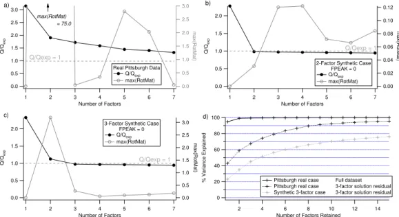
Q-values and maximum value of RotMat for the real Pitts-burgh dataset for solutions up to 7 factors are shown in Fig. 3a and mass fractions of these solutions are shown in Fig. 4a, all for FPEAK=0. There is a large drop in the
Q/Qexp value from one to two factors, and Q/Qexp is 1.9
at 2 factors. Additional factors continue to reduceQ/Qexp
toward 1, but no strong change in slope is observed (largest steps are 9% from 2–3 factors and 4–5 factors). With seven factors,Q/Qexpis 1.3. TheQcriterion clearly implies that
at least two factors are necessary to explain the data, but there is no strong indication for choosing another solution. Max(RotMat) has a distinct maximum at 2 factors and much smaller values for larger numbers of factors. There is a local minimum at 3 factors and another at 7 factors (confirmed by solutions with>7 factors). Based on the trends ofQ/Qexp
3.0 2.5 2.0 1.5 1.0 0.5 0.0 Q/ Qex p 7 6 5 4 3 2 1
Number of Factors
3.0 2.5 2.0 1.5 1.0 0.5 0.0 max (RotMat )
Q/Qexp = 1 max(RotMat)
a)
= 75.0
Real Pittsburgh Data Q/Qexp max(RotMat) 2.0 1.5 1.0 0.5 0.0 Q/ Qex p 7 6 5 4 3 2 1
Number of Factors
0.12 0.10 0.08 0.06 0.04 0.02 0.00 max (RotMat )
Q/Qexp = 1
b)
2-Factor Synthetic Case FPEAK = 0 Q/Qexp max(RotMat) 2.0 1.5 1.0 0.5 0.0 Q/Q exp 7 6 5 4 3 2 1
Number of Factors
3.0 2.5 2.0 1.5 1.0 0.5 0.0 max( Rot M at)
Q/Qexp = 1
c)
3-Factor Synthetic Case FPEAK = 0 Q/Qexp max(RotMat) 100 80 60 40 20 0 % Varianc e Explained 14 12 10 8 6 4 2
Number of Factors Retained
d)
Pittsburgh real case Full dataset Pittsburgh real case 3-factor solution residual Synthetic 3-factor case 3-factor solution residual
Fig. 3.Values ofQ/Qexpand the maximum value of RotMat for(a)the real Pittsburgh case,(b)the two-factor synthetic case, and(c)the three-factor synthetic case.(d)Percent variance explained by factors from SVD analysis of the Pittsburgh real data matrix and the residual matrices from the Pittsburgh real case solution with 3 factors and the synthetic 3-factor base case solution with 3 factors.
1.0 0.8 0.6 0.4 0.2 0.0 Frac ti on of M a ss
2 3 4 5 6
Number of Factors in PMF Solution
a) Pittsburgh Real Case
PMF Factors Residual OOA-1 OOA-1_a OOA-2 "mixed" HOA_a HOA 1.0 0.8 0.6 0.4 0.2 0.0 F rac ti
on of M
a
s
s
Input 2 3 4 5 6 7
Number of Factors in PMF Solution
b) 2-Factor Synthetic Base Case
Input Factors HOA OOA PMF Factors Residual OOA_a OOA_b OOA_c mixed_a mixed_b HOA_b HOA_a 1.0 0.8 0.6 0.4 0.2 0.0 F rac tion of M a s s
Input 2 3 4 5 6 7
Number of Factors in PMF Solution
c) 3-Factor Synthetic Base Case
Input Factors OOA-1 OOA-2 HOA PMF Factors Residual OOA-1_a OOA-1_b OOA-1_c OOA-2 HOA_a HOA_b HOA_c
each solution stepwise and attempt to interpret them based on correlations with reference MS and tracer TS and use this interpretability as a guide for choosing the number of factors. 2-factor solution
The MS and TS of the two-factor solution are shown in Fig. S3a, see http://www.atmos-chem-phys.net/9/2891/ 2009/acp-9-2891-2009-supplement.pdf. These two factors reproduce the MS and TS found by Zhang et al. (2005a) for this dataset using their original 2-component CPCA method (UCMSHOA Zhang,HOA PMF=0.98, UCMSOOA Zhang,OOA PMF>0.99, UCTSHOA Zhang,HOA PMF=0.9, UCTSOOA Zhang,OOA PMF>0.99) at FPEAK=0. The OOA factor has 12%m/z44 and the HOA factor has 3%m/z44 at FPEAK=0. All interpretations of the factors made by Zhang et al. (2005a, c) hold for these factors. 3-factor solution
The MS and TS of the three factor solution at FPEAK=0 are shown in Fig. 5 (correlations between selected PMF and tracer TS are shown in Table S1, see http://www.atmos-chem-phys.net/9/2891/2009/ acp-9-2891-2009-supplement.pdf). The three-factor solu-tion has HOA and OOA factors very similar to the Zhang et al. (2005a) HOA and OOA (UCMSHOA Zhang,HOA PMF=0.97, UCMSOOA Zhang,OOA PMF>0.99; UCTSHOA Zhang,HOA PMF>0.99,
UCTSOOA Zhang,OOA PMF=0.98) that correlate well with primary
combustion tracers (UCTSCO,HOA=0.93, UCTSNO
x,HOA=0.95) and AMS sulfate (UCTSSulfate,OOA=0.95), respectively. Note that HOA likely encompasses both gasoline and diesel engine emissions, plus other sources of reduced aerosols such as meat cooking (Mohr et al., 2009). PMF analysis of molecular markers results in a similar phenomenon in which the composition of gasoline and diesel emissions are too similar and a factor representing the sum is often retrieved (Brinkman et al., 2006).
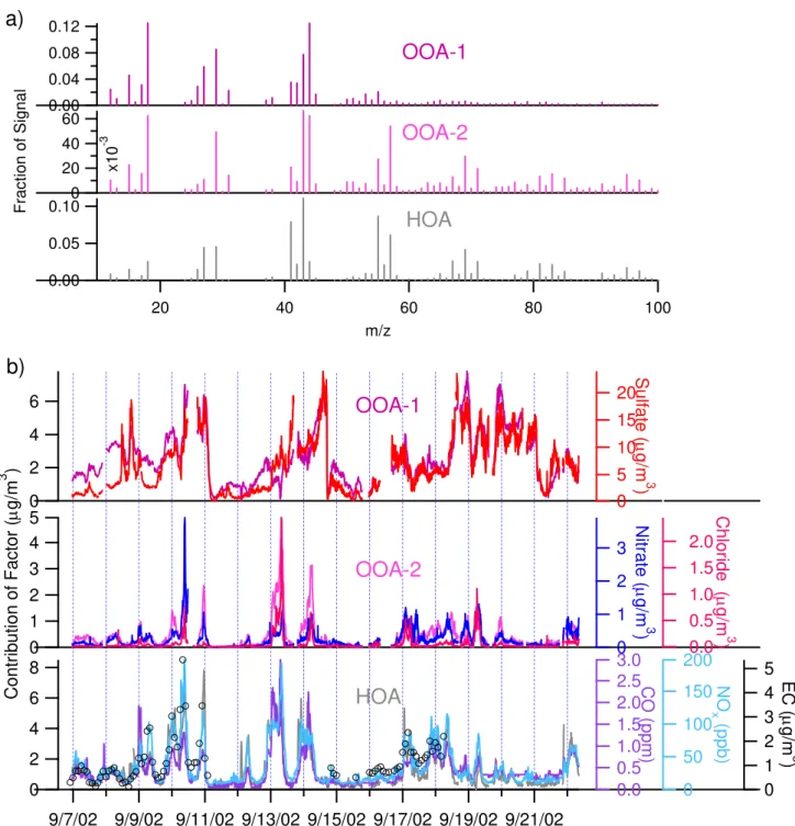
The third factor represents 10% of the OA mass and has a MS with strong correlation with several primary, secondary, and biomass burning OA spectra from the AMS Spectral Database (Figs. 6a, S4a, Ta-ble S2, see http://www.atmos-chem-phys.net/9/2891/2009/ acp-9-2891-2009-supplement.pdf). We identify this spec-trum as a second type of OOA, OOA-2, because of the strong presence of m/z44 (high resolution aerosol mass spectrometer data of ambient aerosols confirm that this is most likely CO+2, DeCarlo et al., 2006; Huffman et al., 2009), and the correlation with OOA/SOA spectra. The OOA that accounts for most of the mass is very simi-lar to that identified by Zhang et al. (2005a) and Lanz et al. (2007) and is termed OOA-1, following the nomencla-ture of Lanz et al. (2007). The OOA-2 spectrum lies 23 de-grees out of the HOA/OOA-1 plane (calculation described in Supp. Info, see http://www.atmos-chem-phys.net/9/2891/
2009/acp-9-2891-2009-supplement.pdf), is clearly not a lin-ear combination of the HOA and OOA-1 spectra, and is un-likely to arise due to noise. The lack of significantm/z’s 60 and 73 strongly suggests that this OOA-2 does not arise from a biomass burning source (Alfarra et al., 2007; Schnei-der et al., 2006). The OOA-2 time series correlates well with ammonium nitrate and ammonium chloride from the AMS, two secondary inorganic species which were not in-cluded in the PMF analysis (UCTSAmmonium Nitrate,OOA−2=0.79,
UCTSAmmonium Chloride,OOA−2=0.82; diurnal cycles are shown
in Fig. S5, see http://www.atmos-chem-phys.net/9/2891/ 2009/acp-9-2891-2009-supplement.pdf). Note that we can confirm that nitrate and chloride signals from the AMS in this study are indeed dominated by the inorganic ammo-nium salts, not fragments of organic species, based on the ammonium balance (Zhang et al., 2005b, 2007b). The OOA-2 factor is less-oxygenated than OOA-1 and more oxy-genated than HOA (m/z44 of 1 is 12.5%, of OOA-2 is 6%, and of HOA is OOA-2.5%). Since both nitrate and chloride show a semivolatile behavior in Pittsburgh (Zhang et al., 2005b), these correlations imply that OOA-2 is also semivolatile. Most likely OOA-2 corresponds to less oxi-dized, semivolatile SOA, while OOA-1 likely represents a more aged SOA that is much less volatile. Direct volatil-ity measurements with a thermal-denuder AMS combina-tion indeed show that in Mexico City and Riverside, CA, the less oxygenated OOA-2 component is more volatile than the OOA-1 component (Huffman et al., 2009). A similar OOA-2 factor with a less oxidized spectrum and a high cor-relation with nitrate was reported by Lanz et al. (2007) for their dataset in Zurich in summer of 2005, though the ra-tios of OOA-2 to nitrate differ (∼1 in the present work,∼2 in Zurich). These authors also interpreted OOA-2 as fresh SOA. No evidence is available to support the identification of OOA-1 or OOA-2 as either “anthropogenic” or “biogenic” in origin.
4-factor solution
The TS and MS for the 4-factor solution are shown in Fig. S3b, see http://www.atmos-chem-phys.net/ 9/2891/2009/acp-9-2891-2009-supplement.pdf. The four-factor solution has clear HOA, OOA-1, and OOA-2 factors with high similarity to those in the 3-factor case (UCTS3−factor OOA−1,4−factor OOA−1=0.96, UCMS3−factor OOA−1,4−factor OOA−1=0.99;
UCTS3−factor OOA−2,4−factor OOA−2, UCMS3−factor OOA−2,4−factor OOA−2>0.99; UCTS3−factor HOA,4−factor HOA,
UCMS3−factor HOA,4−factor HOA>0.99) which are
0.12
0.08
0.04
0.00
100 80
60 40
20
m/z 0.10
0.05
0.00
Fra
c
tion o
f Sign
al
60 40 20 0
x10
-3
HOA
OOA-1
OOA-2
a)
6
4
2
0
9/7/02
9/9/02 9/11/02 9/13/02 9/15/02 9/17/02 9/19/02 9/21/02
8
6
4
2
0
Contr
ib
u
tion
of F
a
ctor
(
µ
g/m
3
)
5
4
3
2
1
0
3
2
1
0
Ni
tra
te (
µ
g/
m
3
)
2.0
1.5
1.0
0.5
0.0
Chlor
ide (
µ
g/m
3
)
20
15
10
5
0
Sulfat
e (
µ
g/m
3
)
3.0
2.5
2.0
1.5
1.0
0.5
0.0
CO (
ppm
)
200
150
100
50
0
NO
x
(p
p
b
)
5
4
3
2
1
0
EC (
µ
g/m
3
)
0.00
O
x
(
ppb)
HOA
OOA-1
OOA-2
b)
Fig. 5.Factors from the three-component PMF solution of the real Pittsburgh dataset for FPEAK=0.(a)Mass spectra of the three components. The fraction of the signal abovem/z100 is 3.4%, 24.3%, and 9.7% for OOA-1, OOA-2, and HOA, respectively.(b)Time series of the three components and tracers.
UCMSdatabase spectra,4−factor Unnamed>0.8 with database mass spectra of the Zhang Pittsburgh OOA, three types of SOA, and four types of biomass burning (Figs. 6b, S4b, Table S2, see http://www.atmos-chem-phys.net/9/2891/ 2009/acp-9-2891-2009-supplement.pdf). However, strong independent evidence (such as a strong tracer correlation)
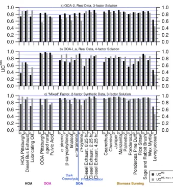
1.0 1.0 0.8 0.8 0.6 0.6 0.4 0.4 0.2 0.2 0.0 0.0 UC MS HOA P itts burgh a D iesel Bu s Exh a u st b Lub ric a tin g Oil b OOA P itts burgh a age d rural c Fulv ic Ac id d α -p ine n e e β -caryop h y lle ne e linalool e α -t erp ine ne e m -xy le n e e Di es el E x h aus t, 0 .25 hr f Di es el E x h aus t, 2 .25 hr f Di es el E x h aus t, 4 .25 hr f Ce an othu s g Chamise g Juniper g Ma nz ani ta g Pa lm et to g Po nd eros a g Ponderos a P ine Duff g Ri ce Straw g S age an d Rabb it B rus h g Wax Myrt le g Lev og luc o s a n h 1.0 1.0 0.8 0.8 0.6 0.6 0.4 0.4 0.2 0.2 0.0 0.0 1.0 1.0 0.8 0.8 0.6 0.6 0.4 0.4 0.2 0.2 0.0 0.0
HOA OOA Biomass Burning
a) OOA-2, Real Data, 3-factor Solution
b) OOA-I_a, Real Data, 4-factor Solution
c) "Mixed" Factor, 2-factor Synthetic Data, 3-factor Solution
SOA Dark
Ozonolysis Photooxidation
UCMS UCMS, m/z > 44
Fig. 6. UCMS between representative spectra from the AMS Mass Spectral Database (http://cires.colorado.edu/jimenez-group/ AMSsd) and(a)the third factor mass spectrum from the 3-factor PMF solution of the real Pittsburgh dataset,(b) the fourth factor mass spectrum from the 4-factor PMF solution of the real Pitts-burgh dataset, and(c)the “mixed” factor mass spectrum from the 3-factor PMF solution of 2-factor base case. Values are given in Table S1 (see http://www.atmos-chem-phys.net/9/2891/2009/ acp-9-2891-2009-supplement.pdf). Superscripts denote the source of the reference spectra as follows: (a)Zhang et al., 2005a; (b) Canagaratna et al., 2004;(c)Alfarra et al., 2004;(d)Alfarra, 2004; (e)Bahreini et al., 2005; (f)Sage et al., 2007;(g)I. M. Ulbrich, J. Kroll, J. A. Huffman, T. Onash, A. Trimborn, J. L. Jimenez, un-published spectra, FLAME-I, Missoula, MT, 2006;(h)Schneider et al., 2006.
absence of any supporting evidence, we concluded that this component represents an artificial “splitting” of the solution (calling this factor OOA-1a) and that keeping this compo-nent would be an overinterpretation of the PMF results. In particular we warn about trying to interpret e.g. one of the OOA-1’s as “biogenic” and the other as “anthropogenic” or similar splits, in the absence of strong evidence to support these assignments.
Five and more factor solutions
The five-factor solution (Fig. S3c, see http: //www.atmos-chem-phys.net/9/2891/2009/
acp-9-2891-2009-supplement.pdf) has four factors that are similar (OOA-1, OOA-1a, OOA-2, HOA) (UCTS4−factor,5−factor>0.96, UCMS4−factor,5−factor>0.90) to the factors in the 4-factor solution. The fifth
factor (HOA a) is similar to the HOA factor in this solution (UCMS5−factor HOA,5−factor HOA a=0.85,
UCTS5−factor HOA,5−factor HOA a=0.68) and has
UCMSDatabase Spectra,5−factor HOA a>0.8 with five types of SOA and eight types of BBOA, but there is no strong correlation with any available tracer. The HOA and HOA a factors have 23% and 15% of the mass, respectively. As before, we conclude that this “splitting” of the HOA is most likely a mathematical artifact and not a real component.
Interpretation of factors in the six- and seven-factor solu-tions becomes more complex and no independent informa-tion from tracer correlainforma-tions exists to substantiate the inter-pretation of these factors. These factors likely arise due to splitting of the real factors, likely triggered by variations in the spectra of the real components (discussed below). Uncertainty of the solutions of real data
In order to explore the possibility of multiple local minima in the solutions of the dataset and qualitatively assess variability in the factors, trials with 64 multiple starts were calculated for the real Pittsburgh case with solutions up to 6 factors. Local minima can be identified by solutions with different
Q/Qexpvalues, but this is not a sufficient criterion as it could
be possible for two local minima to have similarQ/Qexp
val-ues with different factors; therefore similarity of the factor MS and TS is also considered as a criterion for determining local minima. In the solutions with 2- to 6-factors, no lo-cal solutions were observed. The 3-factor solutions show the greatest variation inQ/Qexpvalues, which however increase
by only 2×10⁻⁴Q/Qexp units above the minimum. There
are two modes of the solutions in this small range, defined by the ratio ofm/z43:m/z44 in the MS of the OOA-2 factor, while the MS of the OOA-1 factor varies little and the MS of the HOA factor is virtually identical in all solutions. The TS of all of these solutions are virtually identical (the overlaid TS and MS of all 64 solutions for the 3–5 factor solutions are shown in Fig. S6, see http://www.atmos-chem-phys.net/ 9/2891/2009/acp-9-2891-2009-supplement.pdf).
25
20
15
10
5
0
Q/Q
ex
p
, Real case
9/11/2002
9/16/2002
9/21/2002
8
6
4
2
0
Q/Q
exp
, 2- 3-f
a
ct
o
r S
y
n so
ln
60
40
20
0
Q/Q
exp
,
1-facto
r Syn so
ln
6
4
2
0
OO
A-1 (
µ
g/m
3
)
5
4
3
2
1
0
OO
A-2
(
µ
g/
m
3
)
8
6
4
2
0
HOA (
µ
g/
m
3
)
Q = Qexp
Q=Qexp
a)
b)
c)
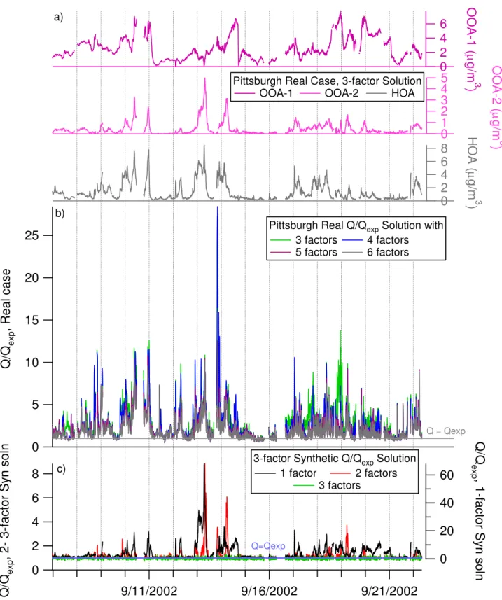
Pittsburgh Real Q/Qexp Solution with
3 factors 4 factors
5 factors 6 factors
Pittsburgh Real Case, 3-factor Solution
OOA-1 OOA-2 HOA
3-factor Synthetic Q/Qexp Solution
1 factor 2 factors
3 factors
16
12
8
4
0
-4
-8
-12
Scal
e
d
R
e
si
dua
l (
eij
/
σij
)
300 280 260 240 220 200 180 160 140 120 100 80 60 40 20
m/z a)
-4 -3 -2 -1 0 1 2 3 4
Scal
e
d
R
e
si
dua
l (
eij
/
σij
)
300 280 260 240 220 200 180 160 140 120 100 80 60 40 20
m/z b)
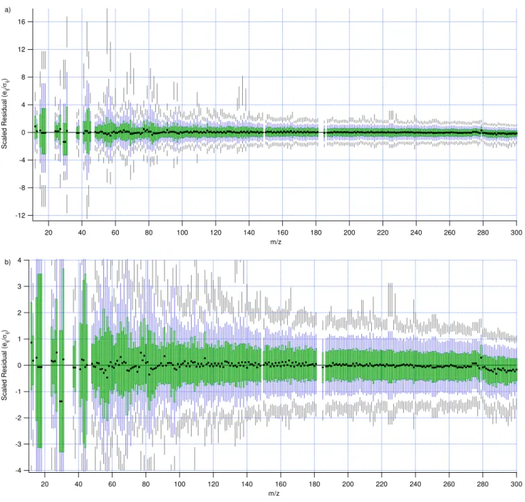
Fig. 8. (a)Distributions of scaled residuals for eachm/zfor the 3-factor solution of the real Pittsburgh case. Black markers represent medians. Green boxes span the 25th and 75th percentiles; blue whiskers attached to the boxes extend to 10th and 90th percentiles. Grey “floating” whiskers connect 2nd to 5th percentiles and 95th to 98th percentiles.(b)Expansion of (a) showing the scaled residuals from−4 to 4.
Residuals of the PMF solutions
Figure 7 shows the Q/Qexp values for each point in time
and Fig. S8 shows the total residuals (6 residual), total absolute residuals (6|residual|), and normalized absolute residuals (6|residual|/6 signal|) for the 3- through 6-factor solutions for FPEAK=0. Note that Qexp for a
time sample equals the number of m/z’s in the MS (268). Figure 8 shows a summary distribution of the scaled
residuals for all m/z from the real Pittsburgh data and Fig. S9 shows the distribution of the scaled residuals for selected m/z’s (see http://www.atmos-chem-phys.net/9/ 2891/2009/acp-9-2891-2009-supplement.pdf); minimiza-tion of total Q (squared scaled residuals) while meeting non-negativity constraints drives the solutions of the PMF algorithm. The contributions to both Q/Qexp and
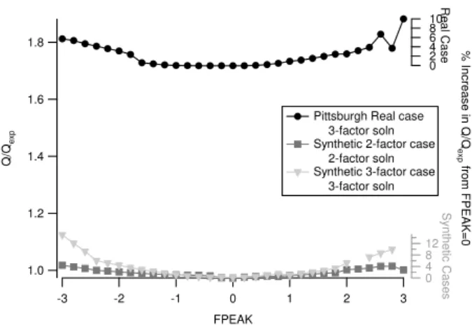
10 8 6 4 2 0
% Inc
reas
e
in Q
/Q
exp
from F
P
EAK=0
-3 -2 -1 0 1 2 3
FPEAK 1.8
1.6
1.4
1.2
1.0
Q/
Qex
p
12 8 4 0
Sy
n
thetic
Cas
e
s
Re
al
Case
Pittsburgh Real case 3-factor soln Synthetic 2-factor case
2-factor soln Synthetic 3-factor case
3-factor soln
Fig. 9.Q/Qexpvs. FPEAK for the real Pittsburgh case with 3 fac-tors, the 2-factor synthetic base case with 2 facfac-tors, and the 3-factor synthetic base case with 3 factors.
is very similar to the OOA-2 time series from the three-factor solution (UCTS3−factorQ/Q
exp,3−factor OOA−2=0.70, UCTS4−factorQ/Q
exp,4−factor OOA−2=0.75, and
UCTS5−factorQ/Q
exp,5−factor OOA−2=0.78). Adding more
factors results in only minor changes in the TS ofQ/Qexp
contributions and residual, implying that the same data variation fit by the lower order solution is being refit with more factors. In fact, the decrease in the TS of Q/Qexp
(improvements in the fit) in solutions with 3 to 6 factors do not occur during periods of high HOA or OOA-2, and only occasionally during periods of high OOA-1 (Fig. S10, see http://www.atmos-chem-phys.net/9/2891/ 2009/acp-9-2891-2009-supplement.pdf). The highest spike in the residual TS, a short-lived event on the evening of 14 September 2002, is likely due to a specific HOA plume (e.g., a specific combustion source) whose spectrum is similar to but has some differences from the main HOA factor during the study and shows variation inm/zpeaks with higher con-tribution to HOA than OOA-2. SVD of the unscaled residual matrix after fitting 3 factors (Fig. 3d) shows that with even 12 more factors, less than 95% of the remaining variance can be explained (150 factors would be needed to explain 95% of the variance in the matrix of scaled residuals that was not downweighted for weakm/z’s or those proportionally related tom/z44). The residual at specificm/z’s during periods of high OOA-2 and highQ/Qexpchanges for many significant
OOA-2m/z’s in modest amounts, fairly continuously, over periods of 10–20 min. This is likely caused by variations in the true OOA-2 spectrum (which could occur, e.g., during condensation or evaporation of SVOCs) that cannot be represented by the constant-MS factor, nor are constant enough to become their own factor. These behaviors imply that three factors have explained as much of the data as is possible with a bilinear model with constant spectra.
3.1.2 Rotations
The three factor solution, which is the most interpretable as discussed above, is tested for its rotational ambiguity. The FPEAK range required for the Q/Qexp=10% criterion
in the real data is−4.2 to +4.4. Solutions with FPEAKs be-tween−1.6 and +1.0 give an increase of 1% overQ/Qexp
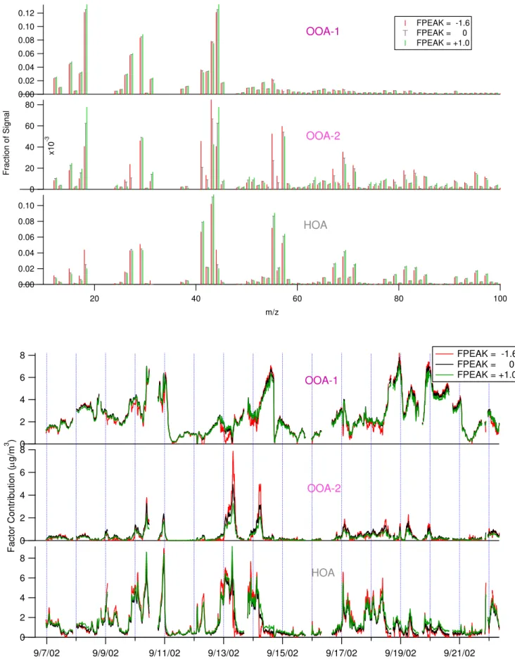
at FPEAK=0 (Fig. 9). MS and TS spanning this range of solutions are shown in Fig. 10. Note that changing FPEAK changes both the MS and TS simultaneously. Overall, the effect of positive FPEAK is to create more near-zero val-ues in the MS and decrease the number of near-zero valval-ues in the TS. The effect of negative FPEAK is to create more zero values in the TS and decrease the number of near-zero values in the MS. Note for example that the TS of the FPEAK=−1.6 solution have periods of zeros that do not cor-relate with any interpretable events, likely indicating that this solution represents rotation beyond the range that gives use-ful insight for this dataset. Changes in TS occur more in some periods than others. Mass concentration of all factors remain fairly constant at all FPEAKs during periods in which at least one factor has a mass concentration near zero, but periods in which all factors have non-zero mass concentra-tions show more variation as FPEAK is changed. This is most dramatic for the OOA-2 events on 13 and 14 Septem-ber 2002, in which negative FPEAKs give more mass to the OOA-2 factor and less mass to the OOA-1 factor compared to solutions with FPEAK≥0. These differences represent one way of characterizing the uncertainty of the PMF solutions, since theQ/Qexpvalues change little between them and all
the TS and MS appear physically plausible. The solutions from multiple FPEAKS (Fig. 10) show a greater range in MS than the bootstrapping 1-σ variation bars, while the TS show a similar range to the bootstrapping 1-σ variation bars (Fig. S7, see http://www.atmos-chem-phys.net/9/2891/2009/ acp-9-2891-2009-supplement.pdf).
The MS change with FPEAK is most dramatic in the OOA-2 MS, while the OOA-1 MS changes very little with FPEAK. This is not surprising since OOA-2 ac-counts for a low fraction of the total signal and thus its spectrum can change more without causing large in-creases in the residuals. At large negative values of FPEAK, the OOA-2 factor strongly resembles the HOA fac-tor (UCMSOOA−2,HOA at FPEAK=−1.6=0.98). The ratio ofm/z43 tom/z44 in OOA-2 decreases from 2.1 to 1.1 and 0.55 as FPEAK increases from−1.6 to 0 and +1.0, respectively. A sharp decrease in the fraction of signal attributed tom/z55 relative to a small decrease inm/z57 (ratios of 0.88, 0.50, and 0 at FPEAKs−1.6, 0, and +1.0, respectively) givesm/z57 an unusually high fraction of the signal in OOA-2 at large positive FPEAKs. Positive FPEAK values also reduce the fraction ofm/z44 (mainly CO+2)attributed to the HOA MS.
0.12
0.10
0.08
0.06
0.04
0.02
0.00
100 80
60 40
20
m/z 0.10
0.08
0.06
0.04
0.02
0.00
F
racti
on
o
f
Si
gn
al
80
60
40
20
0
x10
-3
HOA
OOA-1
OOA-2
FPEAK = -1.6 FPEAK = 0 FPEAK = +1.0
8
6
4
2
0
9/7/02 9/9/02 9/11/02 9/13/02 9/15/02 9/17/02 9/19/02 9/21/02 8
6
4
2
0
Factor
Contr
ibution (
µ
g/m
3 )
8
6
4
2
0
HOA
OOA-1
OOA-2
FPEAK = -1.6 FPEAK = 0 FPEAK = +1.0