www.ocean-sci.net/12/1155/2016/ doi:10.5194/os-12-1155-2016
© Author(s) 2016. CC Attribution 3.0 License.
Acoustic and optical methods to infer water transparency at Time
Series Station Spiekeroog, Wadden Sea
Anne-Christin Schulz1, Thomas H. Badewien1, Shungudzemwoyo P. Garaba2, and Oliver Zielinski1
1Institute for Chemistry and Biology of the Marine Environment, Carl von Ossietzky University of Oldenburg,
Schleusenstr. 1, 26382 Wilhelmshaven, Germany
2Department of Marine Sciences, Avery Point Campus, University of Connecticut, 1080 Shennecosset Road,
Groton, CT 06340, USA
Correspondence to:Oliver Zielinski ([email protected]) Received: 30 April 2016 – Published in Ocean Sci. Discuss.: 30 May 2016
Revised: 22 September 2016 – Accepted: 12 October 2016 – Published: 4 November 2016
Abstract.Water transparency is a primary indicator of opti-cal water quality that is driven by suspended particulate and dissolved material. A data set from the operational Time Se-ries Station Spiekeroog located at a tidal inlet of the Wad-den Sea was used to perform (i) an inter-comparison of ob-servations related to water transparency, (ii) correlation tests among these measured parameters, and (iii) to explore the utility of both acoustic and optical tools in monitoring water transparency. An Acoustic Doppler Current Profiler was used to derive the backscatter signal in the water column. Optical observations were collected using above-water hyperspectral radiometers and a submerged turbidity metre. Bio-fouling on the turbidity sensors optical windows resulted in measure-ment drift and abnormal values during quality control steps. We observed significant correlations between turbidity col-lected by the submerged metre and that derived from above-water radiometer observations. Turbidity from these sensors was also associated with the backscatter signal derived from the acoustic measurements. These findings suggest that both optical and acoustic measurements can be reasonable prox-ies of water transparency with the potential to mitigate gaps and increase data quality in long-time observation of marine environments.
1 Introduction
Over the past decades, scientists, policy makers, and the pub-lic have become more aware of issues of environmental con-cern such as water quality (WFD, 2000; OECD, 1993; Borja
et al., 2013). To better understand the dynamics of water quality, it is necessary to use different platforms and tools, which allow for collecting data over a broad range of tempo-ral and spatial scales (Zielinski et al., 2009; Pearlman et al., 2014). The information from these different tools ought to be comparable for a comprehensive and reliable view of these dynamics. Water quality in general is the state of a water body parameterized according to predefined thresholds typ-ically grouped according to ecological, chemical, optical, or morphological properties. Water transparency is determined from optical observations that involve using the human eye as a tool or methods that replicate the human eye sensing approach (Moore et al., 2009). Optical water quality has been determined for decades as the tools needed are easy to use, fast, inexpensive, and robust. Common optical ob-servations provide information about the light availability in the water column, which can be translated into water trans-parency. Turbidity is one such measurement referring to a relative index of water cloudiness influenced by the inher-ent dissolved and particulate material (Kirk, 1985; Moore, 1980). Another parameter derived from ocean colour remote sensing is remote sensing reflectance (RRS) also known as
an essential climate variable.RRSis a proxy for the apparent
1156 A.-C. Schulz et al.: Acoustic and optical methods to infer water transparency
(indigo-blue) to 21 (cola brown). This information can also be derived fromRRSinformation (Garaba et al., 2014;
Wer-nand and van der Woerd, 2010).
Over the past decades, measurement methods based on acoustic backscatter have been increasingly used to estimate the abundance and distributional patterns of suspended mat-ter (Deines, 1999; Thorne et al., 1991). Indeed, acoustics is one of those technologies advancing our capabilities to probe sediment processes (Thorne and Hanes, 2002; Voul-garis and Meyers, 2004). The acoustic backscatter signal is used to quantitatively determine suspended matter and there-fore relates to turbidity (Deines, 1999; Lohrmann, 2001; Schulz et al., 2015). Therefore, acoustic backscatter sig-nals provide information about the suspended material in a given water body and enable one to record the changes over a long timescale. An Acoustic Doppler Current Profiler (ADCP), for example, measures non-intrusively and three-dimensionally, making it a very powerful tool for examining small-scale sediment transport processes (Thorne and Hanes, 2002; Schulz et al., 2015).
The composition and concentration of suspended material is highly variable in coastal and estuarine regions (Winter et al., 2007; Fugate and Friedrichs, 2002). Fragile floccu-lants change their characteristics over short and over long timescales due to hydrodynamic forcing such as currents, tur-bulence and tides (Vousdoukas et al., 2011; Burchard and Badewien, 2015). Optical (White, 1998; Sutherland et al., 2000) and acoustic methods (Voulgaris and Meyers, 2004; Fugate and Friedrichs, 2002) typically reveal different scat-tering properties of the sediment. Thus, Winter et al. (2007) concluded that the combination of different instruments re-veal different aspects of suspended particulate matter (SPM) dynamics.
The aim of this work is to find out whether measurements of acoustic backscatter can be reliably related to optical wa-ter properties. As all these observations provide information about the inherent suspended particulate and dissolved mate-rial, these should also be suited as practical indicators of wa-ter transparency and thus quality. We also evaluate the utility of acoustic and optical technology in environmental monitor-ing to gather qualitative and quantitative indicators of change within natural waters taking advantage of operational long time series observatory platforms. The goals of this study will be towards (i) inter-comparison of measurements from different tools, (ii) understanding correlations among the ob-served variables, and (ii) developing methods geared to clos-ing gaps in relevant information about variability in water transparency in the water column such as when individual instruments fail.
2 Materials and methods 2.1 Study area
Time Series Station Spiekeroog (TSS; Fig. 1) is a mul-tidisciplinary, autonomously operating observatory located in a tidal channel between the islands of Langeoog and Spiekeroog at 53◦
45.016′
N, 7◦
40.266′
E (Reuter et al., 2009). These islands are part of an island barrier system in the East Frisian Wadden Sea, southern North Sea, which be-longs to the UNESCO World Natural Heritage sites. The re-gion is part of an extended North Sea tidal flat system with shallow water depths ranging from 0 to 20 m, with current velocities of up to 2 m s−1. The tidal cycle is semi-diurnal.
The water depth at the TSS Spiekeroog is about 13.5 m, with a tidal range of about 2.7 m (Holinde et al., 2015). Here, the distribution of suspended particulate inorganic and organic material is strongly influenced by tidal currents as well as by wind-driven waves (Bartholomä et al., 2009; Badewien et al., 2009). Because of these strong and rapid dynamics, the area at the TSS is well suited for studying the biogeochemical and physical processes occurring at the transition from the coast to the open sea.
2.2 Sampling and analysis
Hyperspectral radiometers were used to collect and derive
RRS data at 24 m above the seafloor at 5 min interval
con-tinuously. The reflectance measurements, corrected for en-vironmental perturbations, were transformed into Forel–Ule colour indices that can be matched to the intrinsic colour of water. A submerged WETlabs ECO FLNTU sensor mea-sured turbidity at 12 m above the seafloor continuously at 1 min intervals. The ECO FLNTU sensor samples turbidity data with optical backscattering at a wavelength of 700 nm. Detailed information on the processing of these measure-ments is presented in an earlier study from Garaba et al. (2014).
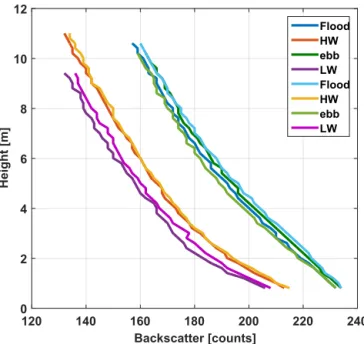
A bottom-mounted (1.5 m above the seafloor), up-ward looking 1200 kHz ADCP (Teledyne RD Instruments Workhorse Sentinel, USA) was used to estimate the current velocity using the Doppler effect in three dimensions. The ADCP is installed at a distance of 12 m north-north-west of the station’s pole. We receive data over the entire water depth with a vertical resolution of 0.20 m (bin size) and a tempo-ral resolution of 5 min (measurements are averaged over 45 pings in 5 min bursts). The shape of the depth profiles de-rived from the backscatter data (Fig. 2) vary depending on the tidal phase (flood, ebb, slack water). Those phases with similar current velocity also result in similar shapes of the backscatter profiles. Because the ADCP has a beam angle of 20◦
and a tilted orientation with a pitch of∼19.39◦and a roll
of∼17.96◦, the maximum rangeRmaxin metres of
accept-able data is given by
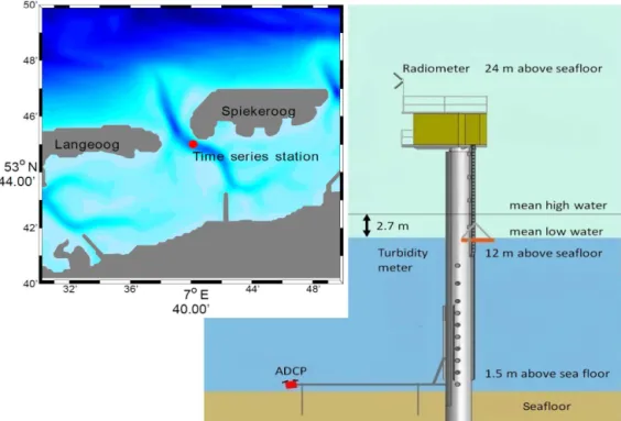
Figure 1.Schematic of the Time Series Station Spiekeroog showing the position of the radiometers (24 m), the turbidity metre (12 m), and the ADCP (1.5 m above the seafloor). The typical water depth is 13.5 m with tidal range of about 2.7 m between mean high and low water. The insert shows the location of the Time Series Station where the colours indicate the water depth at high water.
whereDis the distance between the ADCP and the surface in metres, and φ is the angle in degrees of the beam rela-tive to the vertical. The resulting blank space near the sur-face reached values between 3.0 and 3.5 m (see Fig. 3). To compare the data at nearly the same sampling target, we ex-trapolate the acoustic backscatter signal to the sea surface area (details of the sampling areas of the different sensors are shown in Fig. 4), using the acceptable acoustic backscatter data untilRmaxdepth. To do so, we applied various curve
fit-ting techniques using MATLAB R2015a Curve Fitfit-ting Tool-box (MathWorks, USA). These methods were (i) the expo-nential fitting method (exp, equation: a·exp(b·x)), (ii) the polynomial fitting method (poly, equation:p1·x+p2, basi-cally linear), (iii) the power fitting method (power, equation:
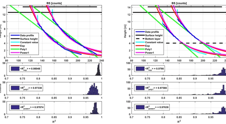
a·xb), and (iv) constant extrapolation (using the last reliable data value as the surface value). Applications of these meth-ods are shown in Fig. 5. The top panels show profiles, which are exemplary for data obtained during low water and one during flooding (violet and blue in Fig. 2) with different ex-trapolations to the surface layer. These panels also demon-strate the different ranges that were used for extrapolating; data were extrapolated using measurements obtained within the entire water column (left panel). In an alternative ap-proach, extrapolation of data was based solely on measure-ments not affected by bottom friction – that is data derived in the near-bottom range up to 4 m were excluded (right panel). In this range, the impact of ebb- and flood-induced currents is strong. The bottom panel shows the summary of allR2
ob-tained from the different extrapolation methods on the entire data set. We assume that the distribution of suspended matter near the surface layer is nearly homogeneous (e.g. Badewien et al., 2009; van der Hout et al., 2015) because of turbulence and wind influence.
The exponential extrapolation (exp) resulted in the best fits for all data sets and extrapolation ranges. TheR2values over the entire period are good withR2>0.99 (see Fig. 5, bot-tom). Therefore, to compare acoustic backscatter data with the other parameters, the exponential fitting method and the extrapolations with constant values (BSEx,expand BSEx,const)
were used. The latter was based on the assumption of homo-geneity in the top layer of the water column.
3 Results
1158 A.-C. Schulz et al.: Acoustic and optical methods to infer water transparency
Backscatter [counts]
120 140 160 180 200 220 240
Height
[m]
0 2 4 6 8 10 12
Flood HW ebb LW Flood HW ebb LW
Figure 2. Example acoustic backscatter profiles measured from ADCP over height in counts observed on 29 August 2013 at dif-ferent tidal phases: flood, ebb, slack water (high water (HW), low water (LW)).
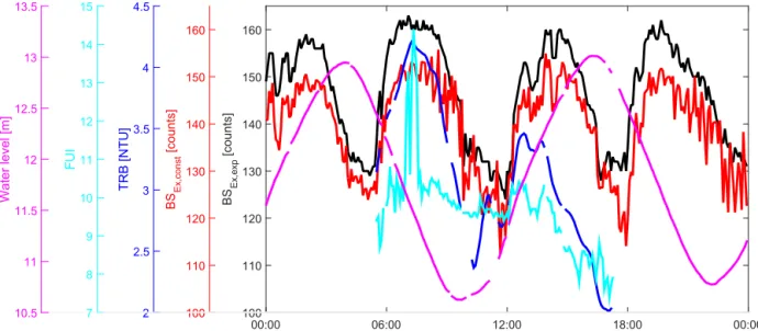
indicate that the upper limit of reliable measurements had been reached. Figure 7 presents a closer look at the variables of the acoustic and optical measurements obtained on 29 Au-gust 2013. Visual inspection of data (Forel–Ule index, turbid-ity and the acoustic backscatter) suggested that there was a moderate correlation. As expected, the highest values of the variables investigated were during periods with high current speeds, i.e. when the water level rises or falls. Because of the measurement principle the Forel–Ule index was restricted to a time span between 06:00 and 18:00 resulting from day-time and the reflectance of the sunlight. The signals of both the Forel–Ule index FUI and the turbidity TRB were stronger during ebb tide than during flood tide. The acoustic backscat-ter signals, which were extrapolated using constant values BSEx,const, were nearly equal strength during ebb and flood
tide, whereas BSEx,exp exhibited stronger ebb signal.
How-ever, during slack water the values were slightly decreasing. Thus, the dynamics of all data sets corresponded well to the observed tidal signal.
Results of the Spearman rank correlation for 1 day (29 Au-gust 2013, directly after sensor cleaning) and for a longer pe-riod (5 days) are shown in Table 1. As described above, we extrapolated the acoustic backscatter signal towards the sea surface to be able to compare these acoustic measurements with the optical approaches. Two of these extrapolated vari-ables (BSEx,const and BSEx,exp) were used for the Spearman
rank correlation test. The correlation coefficient between the data sets increased from moderate (ρSpearman>0.4 and
ρSpearman<0.6) to strong (ρSpearman>0.6 and ρSpearman<
0.8). In general, the correlation values of the shorter time pe-riods were higher, than the values for the longer time period, especially for the comparison of the acoustic backscatter sig-nal and the turbidity. The correlation between FUI and TRB was also very good (ρSpearman>0.8). The comparison of the
two different time periods showed nearly the same values. For further investigations, we used the constant extrapolated acoustic backscatter signal BSEx,const. For this approach, we
assumed a homogenous surface layer (see above).
Table 2 shows a comparison between the constantly ex-trapolated ADCP backscatter signal BSEx,constand the Forel–
Ule index and the turbidity data separated into different tidal phases: ebb, flood, high waters, low waters. The data cover the time period from 29 August 2013 to 2 Septem-ber 2013. The correlations between the acoustic backscatter data BSEx,const and FUI ranged from a weak correlation of
ρSpearman=0.34 during high tide to a strong correlation
dur-ing low tide of ρSpearman=0.81. In between, the methods
correlated mostly moderate (ρSpearman>0.4 andρSpearman<
0.6). The correlations between acoustic backscatter data BSEx,const and TRB were weak at high tide and flood, and
otherwise strong (ρSpearman>0.6 andρSpearman<0.8).
4 Discussion
The time series of turbidity data shown in Fig. 6 indicate the strong influence of fouling on the sensors during the bio-active seasons spring and summer even during shorter time periods of several days. Thus, it is vital to regularly check and, if necessary, clean sensors to reduce the impact of bio-fouling on data quality. The merely moderate correlation be-tween the acoustic backscatter data BSEx,constand the Forel–
29.8.2013
00:00:00 06:00:00 12:00:00 18:00:00
Height [m]
0 2 4 6 8 10 12 14 16 18
Surface height [m] Rmax[m]
Counts
140 150 160 170 180 190 200 210 220 230 240 BS
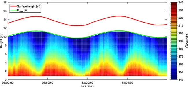
Figure 3.An example of acoustic backscatter signal in counts measured with the ADCP (from the seafloor upwards through the water
column), acceptable backscatter data untilRmax. Green line:Rmaxdepth in metres; red line: sea level (height in metres) observed on
29 August 2013.
Figure 4.Schematic of the different measurement fields of view (FOV) of the sensors at the Time Series Station Spiekeroog at high water. Left panel: top view; right panel: perspective from south (provided by Nick Rüssmeier).
modelling study by Stanev et al. (2007) showed different sediment concentrations and dynamics for fine SPM (mud,
dmud=63 µm; d: diameter) and sand (dsand=200 µm) for
this Wadden Sea area. Depending on the specific location, the dynamics of the different sediment types (fine or coarse) act differently dependent on the tidal signal. Concentrations of coarser material usually clearly peak at maximum flow ve-locities (flood and ebb). The concentration of fine sediments is the highest during ebb, although the peak is broader. The peak during flood is less pronounced. In this study, the dy-namics observed in all data sets corresponds well to the
ob-served tidal signal (Fig. 7). As shown in Schulz et al. (2015) the remaining shear currents in the surface layer kept parti-cles within the water column at slack water times. Thus, we assume that the instruments used in this study provide rea-sonable proxies for suspended material which is comparable in size.
1160 A.-C. Schulz et al.: Acoustic and optical methods to infer water transparency
x
80 100 120 140 160 180 200 220 240
Height
[m]
0 2 4 6 8 10 12 14
BS [counts]
Data profile Surface height Constant value Exp Poly1 Power1
x
80 100 120 140 160 180 200 220 240
Height [m]
0 2 4 6 8 10 12 14
BS [counts]
Data profile Surface height Bottom layer Constant value Exp Poly1 Power1
0.7 0.75 0.8 0.85 0.9 0.95 1
0 50
<R2 exp> = 0.98948
0.7 0.75 0.8 0.85 0.9 0.95 1
Counts
0 50
<R2poly1> = 0.97338
R2
0.7 0.75 0.8 0.85 0.9 0.95 1
0 50
<R2
power1> = 0.97874
0.7 0.75 0.8 0.85 0.9 0.95 1
0 50 100
<R2 exp> = 0.9766
0.7 0.75 0.8 0.85 0.9 0.95 1
0 50 100
<R2poly1> = 0.97566
R2
0.7 0.75 0.8 0.85 0.9 0.95 1
0 50 100
<R2
power1> = 0.97639
Figure 5.Selected acoustic backscatter profiles during low water and during flooding; top left: extrapolation through the whole water column; top right: extrapolation through the reduced water column. The coloured profiles show the results of the different extrapolation methods (cyan: constant extrapolation; red: exponential extrapolation; green: polynomial extrapolation; magenta: power extrapolation). Black line: surface
layer and black dotted line: lower layer. Bottom panels: histograms of the correspondingR2values (from every profile) for the entire period;
left: for the whole water column, right: for the reduced water column.
29.08.2013–02.09.2013
00:000 00:00 00:00 00:00 00:00 00:00
5 10 15 20 25
Water level [m] TRB
raw[NTU]
TRB [NTU]
Figure 6.Turbidity data in NTU from 29 August 2013 to 2 September 2013, limited in range (0–25 NTU), blue: raw data, red: quality checked data, and green: water level in metres.
correlation test, as shown in Table 1 and 2. The correlation coefficient between the data sets increased from moderate to strong. These differences may result from the different
scat-tering characteristics and dynamics of the kinds of sediment, which occur in this location.
00:00 06:00 12:00 18:00 00:00
B
SE
x,
exp
[count
s]
100 110 120 130 140 150 160
B
SE
x,
const
[count
s]
100 110 120 130 140 150 160
T
RB
[
NT
U]
2 2.5 3 3.5 4 4.5
F
UI
7 8 9 10 11 12 13 14 15
W
at
er
level
[m]
10.5 11 11.5 12 12.5 13 13.5
Figure 7.Time series observations on 29 August 2013 of Forel–Ule colour index (FUI; cyan), backscatter signal (BS; constant extrapolation: red, exponential extrapolation: black), turbidity (blue) and water level (magenta).
Table 1.Spearman rank correlation results of the backscatter data from the ADCP BSEX,constand BSEX,expfor 1 day and for a longer time period (29 August 2013–2 September 2013) as well as the estimated Forel–Ule index FUI and the turbidity TRB.
Variables ρSpearman ρSpearman pvalue pvalue
1 day longer period 1 day longer period
BSEX,constvs. TRB 0.78 0.50 <0.001 <0.001 BSEX,expvs. TRB 0.67 0.42 <0.001 <0.001 BSEX,constvs. FUI 0.58 0.52 <0.001 <0.001 BSEX,expvs. FUI 0.48 0.44 <0.001 <0.001
FUI vs. TRB 0.88 0.85 <0.001 <0.001
Table 2.Spearman rank correlation results of the backscatter data
from the ADCP BSEX,const, the estimated Forel–Ule index FUI, and
the turbidity TRB with separation into tidal phases.
Variables Tide phase ρSpearman pvalue
BSEx,constvs. FUI ebb 0.45 <0.001
flood 0.52 <0.00
high tide 0.34 0.06
low tide 0.81 <0.001
BSEx,constvs. TRB ebb 0.71 <0.001
flood −0.34 <0.001
high tide 0.40 0.0014
low tide 0.77 <0.001
the data of the shorter 1-day time period directly after clean-ing the ECO FLNTU sensor were stronger than the values for the entire time period of 5 days. Even the correlation be-tween the FUI and the TRB was very good and the compari-son of the two different time periods showed nearly the same values. This indicates that both optical measurements (above
and in-water) detect the same type of sediment. In a previous study it was shown that the Forel–Ule index can be used to accurately derive turbidity (Garaba et al., 2014). We there-fore evaluated its potential in providing information about suspended material, which in turn can be compared to in-formation derived from acoustic backscatter signals. Our re-sults regarding the correlation between the acoustic backscat-ter signal and turbidity agree well with the investigations of Schulz et al. (2015). The data sets of the in-water sensors correlated moderately to strongly. In particular, the counter wise strengths of the signals during the tidal cycle could be identified. In summary, our results on the correlation of the different sensor types agree well with previous results from laboratory investigations (Vousdoukas et al., 2011).
5 Conclusions
variabil-1162 A.-C. Schulz et al.: Acoustic and optical methods to infer water transparency
ity in water transparency in the water column when individ-ual instruments fail.
The results of this study show that bio-fouling decreases the data quality of in-water optical measurements of turbid-ity within short time periods. Hence, it is important to find an approach to improve the monitoring over time and increase the robustness of the turbidity results. This study demon-strates that bottom-mounted ADCP measurements, which are hardly influenced by bio-fouling, can be a suitable alternative to overcome the problem. We found that using the acoustic backscatter signal and the Forel–Ule index both yield reliable results, thus broadening the work of Garaba et al. (2014). On a qualitative level, using the Forel–Ule index, as derived from radiometer measurements, is a powerful tool for exchange-able estimations of water transparency as much as data sets derived from ADCP measurements.
We have shown that data sets from different measurement principles (optical and acoustic) are comparable and com-plementary. This is even though the different sensors reveal different scattering properties of particles and are positioned in different ways, i.e. above the sea surface, submerged near the sea surface, and submerged near the seafloor.
Thus, our study strongly suggests that combining these methods can be an effective tool to monitor environmental processes as a part of long time series observatories.
The Supplement related to this article is available online at doi:10.5194/os-12-1155-2016-supplement.
Acknowledgements. We would like to thank Axel Braun, Helmo Nicolai, Gerrit Behrens, and Waldemar Siewert for their ongoing technical assistance and support in all our experimental work and the maintenance of the Time Series Station Spiekeroog. We also thank Constanze Böttcher for English language editing. Thanks to Nick Rüssmeier for CAD illustration. This work has been supported through the Coastal Observing System for Northern and Arctic Seas (COSYNA) funded by the German Federal Ministry of Education and Research through the Helmholtz Association and coordinated by the Helmholtz-Zentrum Geesthacht. We are grateful to the comments from the two anonymous reviewers.
Edited by: R. Dewey
Reviewed by: two anonymous referees
References
Badewien, T. H., Zimmer, E., Bartholomä, A., and Reuter, R.: To-wards continuous long-term measurements of suspended partic-ulate matter (SPM) in turbid coastal waters, Ocean Dynam., 59, 227–238, 2009.
Bartholomä, A., Kubicki, A., Badewien, T. H., and Flemming, B. W.: Suspended sediment transport in the German Wadden
Sea-seasonal variations and extreme events, Ocean Dynam., 59, 213– 225, 2009.
Borja, A., Elliott, M., Andersen, J. H., Cardoso, A. C., Carstensen, J., ao G. Ferreira, J., Heiskanen, A.-S., ao C. Marques, J., ao M. Neto, J., Teixeira, H., Uusitalo, L., Uyarra, M. C., and Zampoukas, N.: Good Environmental Status of marine ecosys-tems: What is it and how do we know when we have attained it?, Mar. Pollut. Bull., 76, 16–27, 2013.
Burchard, H. and Badewien, T. H.: Thermohaline residual cir-culation of the Wadden Sea, Ocean Dynam., 65, 1–14, doi:10.1007/s10236-015-0895-x, 2015.
Deines, K. L.: Backscatter Estimation Using Broadband Acoustic Doppler Current Profilers, in: Current Measurement, 1999, Pro-ceedings of the IEEE Sixth Working Conference on, 249–253, doi:10.1109/CCM.1999.755249, 1999.
Fugate, D. C. and Friedrichs, C. T.: Determining concentration and fall velocity of estuarine particle populations using ADV, OBS and LISST, Cont. Shelf Res., 22, 1867–1886, 2002.
Garaba, S. P. and Zielinski, O.: Comparison of remote sensing re-flectance from above-water and in-water measurements west of Greenland, Labrador Sea, Denmark Strait, and west of Iceland, Opt. Express, 21, 15938–15950, doi:10.1364/OE.21.015938, 2013.
Garaba, S. P., Badewien, T. H., Braun, A., Schulz, A.-C., and Zielin-ski, O.: Using ocean colour products to estimate turbidity at the Wadden Sea time series station Spiekeroog, J. Eur. Opt. Soc.-Rapid, 9, 1–6, doi:10.2971/jeos.2014.14020, 2014.
Garaba, S. P., Voß, D., Wollschläger, J., and Zielinski, O.: Modern approaches to shipborne ocean color remote sensing, Appl. Opt., 54, 3602–3612, 2015.
Gartner, J. W.: Estimating suspended solids concentrations from backscatter intensity measured by acoustic Doppler current pro-filer in San Francisco Bay, California, Mar. Geol., 211, 169–187, 2004.
GCOS: The Global Climate Observing System – Systematic Obser-vation Requirements for Satellite-based Data Products for Cli-mate: 2011 Update GCOS-154, 2011.
Holinde, L., Badewien, T. H., Freund, J. A., Stanev, E. V., and Zielinski, O.: Processing of water level derived from water pres-sure data at the Time Series Station Spiekeroog, Earth Syst. Sci. Data, 7, 289–297, doi:10.5194/essd-7-289-2015, 2015.
Kirk, J. T. O.: Effects of suspensoids (turbidity) on penetration of solar radiation in aquatic ecosystems, Hydrobiologia, 125, 195– 208, 1985.
Lohrmann, A.: Monitoring Sediment Concentration with acous-tic backscattering instruments, nortek technical notes/October15, 2001/Document No. N4000-712, 2001.
Moore, C., Barnard, A., Fietzek, P., Lewis, M. R., Sosik, H. M., White, S., and Zielinski, O.: Optical tools for ocean monitor-ing and research, Ocean Sci., 5, 661–684, doi:10.5194/os-5-661-2009, 2009.
Moore, G. K.: Satellite remote sensing of water turbidity / Sonde de télémesure par satellite de la turbidité de l’eau, J. Eur. Opt. Soc.-Rapid, 5, 407–421, 1980.
Morel, A.: In-water and remote measurements of ocean color, Bound.-Layer Meteorol., 18, 177–201, doi:10.1007/bf00121323, 1980.
En-vironment, Organisation for Economic Co-operation and Devel-opment, Paris, 1993.
Pearlman, J., Garello, R., Delory, E., Castro, A., del Río, J., Toma, D. M., Rolin, J. F., Waldmann, C., and Zielin-ski, O.: Requirements and approaches for a more cost-efficient assessment of ocean waters and ecosystems, and fisheries management, in: 2014 Oceans – St. John’s, 1–9, doi:10.1109/OCEANS.2014.7003144, 2014.
Reuter, R., Badewien, T. H., Bartholomä, A., Braun, A., Lübben, A., and Rullkötter, J.: A hydrographic time series station in the Wadden Sea (southern North Sea), Ocean Dynam., 59, 195, doi:10.1007/s10236-009-0196-3, 2009.
Schulz, A.-C., Badewien, T. H., and Zielinski, O.: Impact of cur-rents and turbulence on turbidity dynamics at the Time Series Station Spiekeroog (Wadden Sea, southern North Sea), IEEE, Current, Waves and Turbulence Measurement (CWTM), 2015 IEEE/OES Eleventh, doi:10.1109/CWTM.2015.7098095, 2015. Stanev, E. V., Brink-Spalink, G., and Wolff, J.-O.: Sediment dynam-ics in tidally dominated environments controlled by transport and turbulence: A case study for the East Frisian Wadden Sea, J. Geo-phys. Res., 112, 1–20, doi:10.1029/2005JC003045, 2007. Sutherland, T., Lane, P., Amos, C., and Downing, J.: The calibration
of optical backscatter sensors for suspended sediment of varying darkness levels, Mar. Geol., 162, 587–597, 2000.
Thorne, P. D. and Hanes, D. M.: A review of acoustic measurement of small-scale sediment processes, Cont. Shelf Res., 22, 603– 632, 2002.
Thorne, P. D., Vincent, C. E., Hardcastle, P. J., Rehmann, S., and Pearson, N.: Measuring suspended sediment concentrations us-ing acoustic backscatter devices, Mar. Geol., 98, 7–16, 1991.
van der Hout, C. M., Gerkema, T., Nauw, J. J., and Ridderinkhof, H.: Observations of a narrow zone of high suspended particulate matter (SPM) concentrations along the Dutch coast, Cont. Shelf Res., 95, 27–38, 2015.
Voulgaris, G. and Meyers, S. T.: Temporal variability of hydrody-namics, sediment concentration and sediment settling velocity in a tidal creek, Cont. Shelf Res., 24, 1659–1683, 2004.
Vousdoukas, M., Aleksiadis, S., Grenz, C., and Verney, R.: Com-parisons of acoustic and optical sensors for suspended sediment concentration measurements under non-homogeneous solutions, J. Coast. Res., 64, 160–164, 2011.
Wernand, M. R. and van der Woerd, H. J.: Spectral analysis of the Forel-Ule Ocean colour comparator scale, J. Eur. Opt. Soc.-Rapid, 5, 10014s, doi:10.2971/jeos.2010.10014s, 2010. WFD: European Water Framework Directive, Directive 2000/60/EC
of the european parliament and of the council, Official Journal of the European Union, L327, 1–72, 2000.
White, T. E.: Status of measurement techniques for coastal sediment transport, Coast. Engin., 35, 17–45, 1998.