Roberto Spinola Barbosa
Member, ABCM [email protected] University of São Paulo Polytechnic School Mechanical Engineering Department São Paulo, SP, Brazil
Vehicle Dynamic Response Due to
Pavement Roughness
The goal of the present study is the development of a spectral method to obtain the frequency response of the half-vehicle subjected to a measured pavement roughness in the frequency domain. For this purpose, a half-vehicle dynamic model with a two-point delayed base excitation was developed to correlate with the spectral density function of the pavement roughness, to obtain the system spectral transfer function, in the frequency domain. The vertical pavement profile was measured along two roads sections. The surface roughness was here expressed in terms of the spectral density function of the measured vertical pavement profile with respect to the evenness wave number of the pavement roughness. A frequency response analysis was applied to obtain the vertical and angular modal vehicle dynamic response with the excitation of the power spectral density (PSD) of the pavement roughness. The results show that at low speed, the vehicle suspension mode is magnified due to the unpaved track signature. At 120 km/h in an undulated asphalted road, the first vehicle vibration mode has a significant motion amplification, which may cause passenger discomfort.
Keywords: vehicle, dynamic, pavement, roughness, random
Introduction1
In general, during the vehicle project and design development phase, the automotive industry utilizes a combination of design tools such as vehicle modal response from numerical simulation (Costa, 1992), laboratory tests with shaker rigs (Boggs, 2009) and the results of experimental field road tests, to fine tune vehicle suspension (Vilela and Tamai, 2005). Despite the efficiency of the numerical simulations, laboratory and experimental tests are still in use, even though being time-consuming, expensive and limited to the specific road conditions of the test track. Quarter car vehicle model with single random input is traditionally used for spectral studies (Barbosa, 2001; Sun, 1998; Cebon, 1999; Silva, 1999). The complete vehicle model is employed for modal and control purpose (Vilela, 2010; Costa 1992). The motivation of the present work is to extend the power of the analytic tools for the design of vehicle suspension with the application of the frequency domain response technique to deal with random input of the pavement roughness. One of the contributions of the present study is the development of a half-vehicle model with delayed two-point base excitation correlated with the spectral density function of a measured pavement roughness, in order to generate the system spectral transfer function in the frequency domain. The vertical pavement profile was measured along two roads sections. The surface roughness is expressed with the spectral density function of the measured vertical pavement profile with respect to the evenness wave number of the pavement roughness. This method allows the identification of the vehicle dynamic response due to the normalized roughness density distribution (or a measured pavement roughness) to address the passenger comfort and vehicle safety due to the pavement/tyre contact load.
Vehicle Modeling
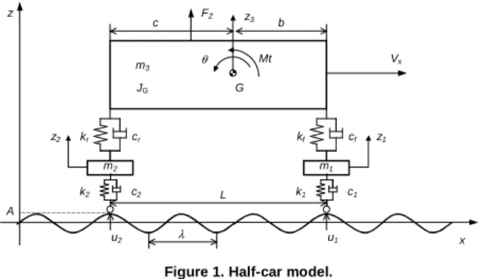
The dynamic vehicle behaviour was accomplished with the traditional half-car vehicle representation (Sun, 2007). The four-degree of freedom lumped parameter model describing relevant motion was adopted as shown at Fig. 1. The vehicle body is free to move vertically in the z3 direction and to acquire an angular motion
θ associated with mass m3 and moment of inertia JG, respectively.
The front and rear suspension connections are described by spring-damper properties (kf, cf, kr and cr). Here m1 and m2 are the vehicle
unsprung mass with the correspondent tyre stiffness and damping
Paper received 6 August 2009. Paper accepted 29 January 2011. Technical Editor: Domingos Rade
are described by k1, c1, k2 and c2 values. The model is excited by the
road evenness u1(t) and u2(t), which induces out-of-phase front and
rear suspension movements, respectively, with a time delay.
x z
Vx
z3
θ
G
λ
L A
u1
u2
b c
m1
m2
JG
z1
z2 kr cr kf cf
k1 c1
k2 c2
Mt FZ
m3
Figure 1. Half-car model.
The equations of motion are obtained using the Lagrange method applied to the lumped rigid bodies. The kinetic, potential and the generalized energy dissipation functions are respectively given by the following equations:
2 2 2 2 1 1 2 2
3 3
2 1 2
1 2
1 2
1
z m z m J
z m
T= & + Gθ& + & + & , (1)
2 20 2 2 2 2 10 1 1 1
2 0 r r 3 r 2 0 f f 3 f
) (
2 1 ) (
2 1
) (
2 1 ) (
2 1
l u z k l u z k
l z b z k l
z b z k V
− − +
− −
+ − − − +
− − +
= θ θ
, (2)
2 2 2 2 2 1 1 1
2 r 3 r 2 f 3 f
) ( 2 1 ) ( 2 1
) (
2 1 ) (
2 1
u z c u z c
z b z c z b z c R
& & &
&
& & & &
& &
− +
−
+ − − +
− +
= θ θ
(3)
J. of the Braz. Soc. of Mech. Sci. & Eng. Copyright 2011 by ABCM July-September 2011, Vol. XXXIII, No. 3 / 303 i i i i i Q q R q V q T q T dt d = ∂ ∂ + ∂ ∂ + ∂ ∂ − ∂ ∂ & & (4)
one obtains the following four differential equations:
0 ) ( ) ( ) ( ) ( 1 3 f 1 3 f 1 1 1 1 1 1 1 1 = − − − − − − − + − + z b z k z b z c u z k u z c z m θ
θ& &
&
& & & &
, (5)
0 ) ( ) ( ) ( ) ( 2 3 2 3 2 2 2 2 2 2 2 2 = − − − − − − − + − + z c z k z c z c u z k u z c z m r
r & θ& & θ
& & & &
, (6)
Z r
r z c z k z c z F
c z b z k z b z c z m = − − + − − + − + + − + + ) ( ) ( ) ( ) ( 2 3 2 3 1 3 f 1 3 f 3 3 θ θ θ θ & & & & & & & &
, (7)
Mt z c z ck z c z cc z b z bk z b z bc J r r z = − − + − − + − + + − + + ) ( ) ( ) ( ) ( 2 3 2 3 1 3 f 1 3 f θ θ θ θ θ & & & & & & & & (8)
Table 1 shows the adopted values for the vehicle inertia, suspension elasticity and dissipation. These values are typical of a medium sized passenger car (Barbosa, 2001).
Table 1. Half-car properties.
Element/Charac. Vehicle Body Suspension Hub/TyreA
Mass 750 kg --- 30 kg
Inertia moment 360 kg m2 ---- ----
RigidityB --- 18.25 kN/m 150 kN/m
Damping --- 912.5 Ns/m ----
Obs.: A
individual properties; B
rigidity depends on the tyre pressure.
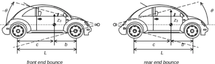
The modal system properties are described by four coupled vibration modes due to the non-diagonal constitution of the system matrix. The vehicle modal response has four natural damped frequencies around 1.0~2.0 and 12 Hz, respectively. For the body modes (front and rear end bounce), as shown in Fig. 2, damping factors are 0.14 and 0.26, respectively, as presented in Table 2. For the suspension modes, associated with the unsprung mass of hub and tyre elasticity, damping factors are around 0.21 as presented in Table 3.
L b c
front end bounce
L b c
z3
rear end bounce z3
−θ θ
Figure 2. Vehicle coupled modes (front and rear end bounce).
It should be noted that the suspension frequency is about one decade above those from the vehicle modes.
The normalized modal Eigen-vectors obtained from the dynamic matrix are shown in the following tables.
Table 2. Vehicle modal properties.
Mode Number Mode 1 – vehicle front end bounce
Mode 2 – vehicle rear end bounce
Damped
Natural Freq 1.03 Hz 1.88 Hz
Damping Factor 0.144 0.261
D. Freedom Mag. Phase Mag. Phase
z1 0.0000 -305.87° 0.0000 -307.44°
z2 0.0002 -203.91° 0.0002 -204.96°
z3 0.0134 -101.95° 1.0000 0.00°
θ 1.0000 0.00° 0.0136 -102.48°
Table 3. Suspension modal properties.
Mode Number Mode 3 – in phase wheel/hub
Mode 4 – out of phase wheel/hub Damped
Natural Freq 11.72 Hz 11.86 Hz
Damping Factor 0.216 0.207
D. Freedom Mag. Phase Mag. Phase
z1 0.0842 -105.13° 0.9880 180.00°
z2 0.9964 0.00° 0.1523 81.712°
z3 0.0006 -315.41° 0.0235 -16.576°
θ 0.0842 -201.27° 0.0036 -114.86°
By taking the Laplace transform of the system equations and assuming zero initial conditions (Felício, 2007), one obtains the four following equations: ) ( ) ( ) ( ) ( ) ( ) ( ) ( )] ( ) ( [ 1 1 1 f f 3 f f 1 f 1 f 1 2 1 s U k s c s bk s bc s Z k s c s Z k k s c c s m + = Θ + + + − + + + + , ) ( ) ( ) ( ) ( ) ( ) ( ) ( )] ( ) ( [ 2 2 2 r r 3 r r 1 r 2 r 2 2 2 s U k s c s ck s cc s Z k s c s Z k k s c c s m + = Θ + + + − + + + + , z F s ck bk s cc bc s Z k s c s Z k s c s Z k k s c c s m = Θ − + − + + − + − + + + + ) ( )] ( ) [( ) ( ) ( ) ( ) ( ) ( )] ( ) ( [ r f r f 2 r r 1 f f 3 r f r f 2 3 , Mt s Z k s c c s Z k s c c s Z k s c b s k c k b s c c c b s JG = + + + − + − Θ − + − + ) ( ) ( ) ( ) ( ) ( ) ( ) ( )] ( ) ( [ 3 r r 2 r r 1 f f r 2 f 2 r 2 f 2 2 (9)
One of the contributions of the present work is the introduction of the delayed out-of-phase inputs into the vehicle front and rear wheels. Considering that the rear wheel runs on the same track right after the front wheel, the surface elevation that produces the vehicle vertical suspension displacement is given by the same function which describes the excitation of the front wheel delayed in time. Taking a harmonic function u1(t) as the imposed vertical
displacement of the front wheel, then the rear wheel delayed input u2(t) can be expressed as:
) ( ) (
2t ut T
u = − , where u1(t)=u(t)=Asin(ωt) (10)
In the above equation ω is the angular frequency given by λ
π
ω=2 Vx/ and T is the time delay given by T=L/Vx, where L
the inter-axis distance, Vx is the vehicle speed and λ is the
The Laplace transformation of the front wheel and the rear wheel input functions, considering the transformation of the delayed function are respectively given by:
)] ( [ )
( 1
1s u t
U =L and U2(s)=L[u2(t)]
where U1(s)=U(s) and U2(s)=U(s)e−Ts (11) Upon the substitution of U(s) into Eq. (11) and the elimination of Z1 and Z2 from these two equations, and after some algebraic
manipulation to get the vertical and angular motions of the vehicle body over displacement excitation U(s) relationship, the following transfer functions for the vertical and angular displacements can be obtained:
) ( ) (
) ( 3
s H s U
s Z
z
= and ( )
) (
) (
s H s U
s Θ = Θ
(12)
The displacement frequency response function (FRF) is known as receptance H(s). However, considering a periodic input, there is a simple relationship between acceleration and displacement, since
) ( )
(t A 2sin t
u&& =− ω ω . The acceleration frequency response function
known as inertance I(s) can be obtained. Analyzing the system vertical and angular forced movements in the frequency domain response, replacing s with (iω) and assuming the vehicle properties presented in Table 1, the frequency response inertance function I(iω) can be obtained as:
) ( )
(
3 3
2 ω
ω
ω H i
i
I&z& = z and IΘ&&(iω)=ω2HΘ(iω) (13)
The vertical ( 3
z
I ) and angular (I ) vehicle modal transfer θ
function depends on T that is a speed function (T=L/Vx). The
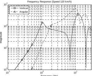
inertance function for the coupled vertical and angular vehicle body motions is shown in Fig. 3. Therefore, the FRF shape will be speed-dependent as can be observed in Fig. 3 for 25.6 km/h (7.1 m/s) and Fig. 4 for 120 km/h (33.3 m/s). In both cases, L = 2.4 m.
10-1 100 101
100 101 102 103
Frequency Response (Speed 25.6 km/h)
Frequency (Hz)
M
a
g
n
it
u
d
e
Vertical Angular
Figure 3. Vehicle inertance frequency response at 25.6 km/h (m3).
Humps can be noticed in the PSD curve shown in Fig. 3 due to the inter-axle distance L (2.4 meters) at a vehicle speed of 25.6 km/h (7.1 m/s). For the vertical mode, these humps occur at every integer, resulting in peaks at around 1, 3, 6, 9 Hz. The modal frequencies are identified with a circle in the figure (front end bounce at 1.03 Hz,
rear end bounce at 1.88 Hz, wheel at 11.7 Hz). For the angular mode, the peaks occur at 13.9, 27.8 Hz etc. (see Fig. 4).
10-1 100 101
100 101 102 103
Frequency Response (Speed 120 km/h)
Frequency (Hz)
M
a
g
n
it
u
d
e
Vertical Angular
Figure 4. Vehicle inertance frequency response at 120 km/h (m3).
It should be pointed out that for a speed of 86 km/h (24 m/s) and an inter-axle distance of 2.4 m, T is equal to 0.1 and, therefore, the next vertical hump is one decade above the frequency of the first mode.
Pavement Roughness Measurement
Two sections of road surface irregularities were actually measured in the present work. The first section was a 1.4 km long road of rustic soil covered with gravel (unpaved road). The second section was a 2.0 km long of asphalted road of high quality. The pavement roughness was measured with the 3-point-middle-chord measuring device. This system is composed of three wheels and a displacement sensor. The two external wheels are steered and the central one is articulated with regard to the others. A conventional car pulls the measuring system along the road measuring the track evenness. The central wheel vertical motion is sampled every centimeter by an analogic to digital sample board installed in a portable computer. The data acquired are stored in magnetic media for post processing purposes (Pavimetro, 2009).
The measured data are treated with the device system transfer function, to obtain the topographic vertical elevation of the road surface roughness, as shown in Fig. 5 for the unpaved road. In this case, ten points per meter were sampled (one sample at every 0.1 meter). Wavelengths up to 200 m were considered.
0 200 400 600 800 1000 1200 1400
-150 -100 -50 0 50 100 150
Road Elevation
Distance (m)
E
le
v
a
ti
o
n
(
m
m
)
fs:10 pto/m T: 100 mm Lambda: 200 m
Pavimetro R
J. of the Braz. Soc. of Mech. Sci. & Eng. Copyright 2011 by ABCM July-September 2011, Vol. XXXIII, No. 3 / 305 The results for the vertical elevation of the road surface roughness
for the asphalted road are shown in Fig. 6. In this case, two points per meter were sampled. Wavelengths up to 500 m were considered in the anti-aliasing processes. The result for the asphalted road evenness is statistically represented by the roughness index unit (International Roughness Index – IRI). The mean IRI value for this road section is 1.92, classified as level A by the ISO criteria.
1500 2000 2500 3000 3500
-150 -100 -50 0 50 100 150
Road Elevation
Distance (m)
E
le
v
a
ti
o
n
(
m
m
)
fs:2 pto/m T: 500 mm Lambda: 500 m
Pavimetro R
IRI 1.92
Figure 6. Highway elevation (asphalt).
The data treatment was performed up to 2048 points at a sample rate down to 10-2 m. This range allows analyzing wavelengths as long as 100 m and down to 0.2 m. This wide range is unprecedented in this area considering that traditional measuring devices have a restricted observable band.
The unpaved and the asphalted track elevation measurements were further treated to generate distributions wavelengths of the periodic irregularities. The spectral density function (PSD) in the range of wavelength between 0.1 to 10 m of the unpaved road vertical elevations is presented in Fig. 7. This measured road section spectrum has its particular signature with intensified wavelength content between 0.4 and 0.9 m.
10-1 100 101
10-12 10-10 10-8 10-6 10-4
Power Spectral Density (Soil)
Wave Length (m)
P
S
D
(
m
3
)
Pavimetro R
Figure 7. PSD of the unpaved track.
The spectral density function of wavelength between 1 and 100 meters of the asphalted vertical elevation road is presented in Fig. 8, where the levels of road roughness intensity are also presented. The spectrum of this road section has its intensified wavelength content between 30 and 40 meters.
100 101 102
10-8 10-7 10-6 10-5 10-4 10-3 10-2 10-1 100
P
S
D
(
m
3
)
Power Spectral Density (Highway)
Wave Length (m)
A B C D E F G H
ISO Class Pavimetro R
Figure 8. PSD of the asphalt pavement.
These measured spectra of vertical elevation of road surface roughness will be used to calculate the vehicle vertical and angular spectral responses. The intensity of the measured pavement roughness is classified, according to the magnitude of the power spectral pattern of the irregularities in an exponential fashion with a particular slope (ISO international standard, 1995). Displacement power spectral density (PSD) for a road roughness class is obtained by a logarithm expression in units of m3:
(
)
ϖo o n n
n Sd n
Sd( )= ( )⋅ / (14)
where the slope in the log-log curve ϖ is fixed at −2 (40 dB per decade). The spatial frequency dependence term Sd at no is obtained from:
0 . 1 4 ) (no = cn+
Sd (15)
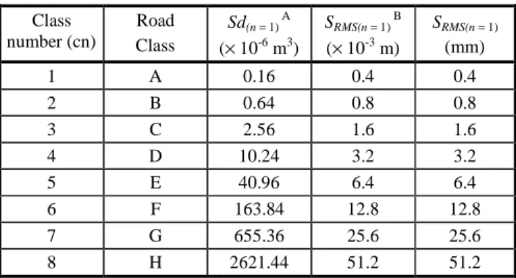
where cn is the class number varying from 1 to 8 (from A to H for different classes of roads, according to ISO). The +1.0 exponent in Eq. (15) applies for the mean geometric roughness for no at 0.1 cycle/m, as shown in Table 4. It should be pointed out that the high quality of the asphalted road section measured is classified as ISO class A, with a Sd(n) wave-length value of 1 meter, given a 16 × 10−8 m3 for the geometric mean and a IRI (International Roughness Index) of 1.92. These values were used as vehicle excitation in the frequency domain.
Table 4. Road Class Roughness.
Class number (cn)
Road Class
Sd(n = 1) A
(× 10-6
m3)
SRMS(n = 1) B
(× 10-3
m)
SRMS(n = 1)
(mm)
1 A 0.16 0.4 0.4
2 B 0.64 0.8 0.8
3 C 2.56 1.6 1.6
4 D 10.24 3.2 3.2
5 E 40.96 6.4 6.4
6 F 163.84 12.8 12.8
7 G 655.36 25.6 25.6
8 H 2621.44 51.2 51.2
Ob.: A
: Geometric Mean; B
: rms value; n = 1 meter, from ISO 8608.
square value (rms-value). According to the Perseval’s theorem (Oppenheim, 1975), the rms-value of a normally distributed random vertical displacement roughness is equal to the square root of the power spectral density. Therefore, by taking the square root of the previous expression, one gets:
(
)
θo o
RMS n Sd n Sd n n n
S ( )= ( )= ( )1/2⋅ / (16)
where the logarithm slope θ changes to −1, which is half of the inclination of Sd (ϖ) (20 dB per decade).
Vehicle/Road Interaction
The vehicle natural behavior is expressed by its frequency domain response function (Barbosa, 1998). The pavement irregularities are expressed by its spatial frequency (1/space). In the present analysis, the road pavement is considered a rigid surface. The relationship between time frequency ω and the spatial frequency n is the vehicle speed V, simply given by:
n V⋅ =
ω (17)
where ω is frequency in Hertz, n = 1/λ is the inverse of the wavelength in meter and V vehicle speed in meters per second. By transforming S(n) into the frequency domain, one gets:
( )
ω ω θω) ( / )
( Sno o
S = ⋅ (18)
According to the theory of stochastic process, the output of a linear time-invariant system is a stationary random process if the input is also a stationary random process. In most cases, the pavement roughness could be described as a zero mean Gaussian ergodic random process (Newland, 1984). Hence, the response of the half-car system is also a zero mean Gaussian stationary random process. The relationship between the PSD of the system response H(ω) and the PSD of the system excitation S(ω) is expressed by:
) ( ) ( )
( 2
3
3 ω H ω Sω
Gz = z and ( ) ( ) ( )
2 ω ω
ω θ
θ H S
G = (19)
where Gz3(ω) and Gθ(ω) are the power spectral densities of the
vehicle vertical displacement responses and the angular response of the sprung mass, respectively.
Vehicle Receptance Response due to track
G(ω) = |H(ω)|2 S(ω)
Vehicle Receptance
H(ω)
output input
Surface Irregularities
S(ω)
Figure 9. Block diagram function.
Applying this transformation to the vehicle inertance function )
( and ) (
3 ω Iθ ω
Iz , the following expressions can be obtained:
) ( ) ( )
(
2 2
3
3ω ω I ω Sω
GI&z& = z&& and ( ) ( ) ( ) 2
2 ω ω
ω
ω θ
θ I S
GI = (20)
The magnitude of the density function of the vertical and angular accelerations of the vehicle riding on the unpaved track at 25 km/h (7 m/s), is shown in Figure 10. It can observed in this figure that the most severe wavelength content of the unpaved track section, which is between 0.4 and 0.9 meters, coincides with the
suspension natural frequency range. This effect magnifies the expected acceleration proneness around 12 Hz, which may cause discomfort to passenger.
100 101
10-12 10-10 10-8 10-6 10-4 10-2 100
Frequency Response (Speed 25.6 km/h)
Frequency (Hz)
M
a
g
n
it
u
d
e
Vertical Angular PSD Track
Figure 10. Vehicle inertance function to unpaved track (m3).
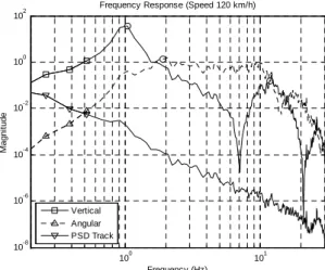
Figure 11 shows the magnitude of the density function of the vertical and angular acceleration of the vehicle riding at 120 km/h on the asphalted road.
100 101
10-8 10-6 10-4 10-2 100 102
Frequency Response (Speed 120 km/h)
Frequency (Hz)
M
a
g
n
it
u
d
e
Vertical Angular PSD Track
Figure 11. Vehicle inertance function in asphalt road at 120 km/h (m3).
A vehicle will be very susceptive to pavement roughness with wavelength content in the range about 2.85 and 34 m (λ=V/ω) whenever traveling at 120 km/h, which will be detrimental to the vehicle performance. Therefore, vehicle suspension tuning process can be optimized against vibrations and a specialized maintenance intervention can produce the best cost/benefit ratio between comfort and the amount of work.
Summary and Conclusions
J. of the Braz. Soc. of Mech. Sci. & Eng. Copyright 2011 by ABCM July-September 2011, Vol. XXXIII, No. 3 / 307 The inertance function is related to the passenger comfort and can be
used for design purposes. The vertical and angular vehicle body transfer functions were calculated with the surface frequency irregularities function in the frequency domain as input.
The first measured road was a 1.4 km long section of an unpaved track and the second was a 2.0 km long section of good quality asphalted road. The geometrical data collected was then processed to obtain a special broadband distribution (with wavelengths between 100 m and 0.2 m) in terms of periodic roughness wavelengths. The wide range of wavelengths thus obtained is unprecedented, considering that the traditional measuring devices have a restricted observable band. The measured asphalted road section has an IRI of 1.92 and can be classified according to ISO criteria as level A. The measured unpaved road section has a spectral signature distribution with concentration between 0.4 and 0.9 m.
A two out-of-phase delayed vehicle inputs was considered corresponding to the front and rear wheel positions, by applying the measured track roughness density functions. The inertance function was obtained for the vertical and angular vehicle body motions. Considering the low speed (25.6 km/h), the vehicle suspension mode is magnified due to the unpaved track signature. In the asphalted track, at high speed (120 km/h), the first vehicle vibration mode has a significant motion amplification, which may cause discomfort to passenger.
The developed methodologies extend the efficiency of vehicle numerical simulation tools, with the power of providing vehicle frequency response analysis due to the pavement roughness statistically described. Results allow the evaluation of passenger discomfort.
A more complex model to address vehicle-pavement interaction can be derived based on a simple four degree of freedom system considered by the present study. Bus, trucks, lorries, complete vehicles and other complex suspension types will be investigated in future researches. For these cases, a two-dimensional pavement auto-correlation roughness function will be necessary. Also, the human comfort behavior according to ISO 2631 may be included in this analysis for the complete cycle of vibration propagation.
Acknowledgements
The author would like to thank the valuable contribution of Professor Edilson Tamai and Marcelo Batista. The author wishes to acknowledge the support to this research provided by the Mechanical Engineering Department of the Polytechnic School – University of São Paulo.
References
Barbosa, R.S., 1998, “Interação Veículo/Pavimento, Conforto e Segurança Veicular”, 31ª Reunião Anual de Pavimentação, Associação Brasileira de Pavimentos – ABPv. Vol. 2, São Paulo, Brazil, pp. 1164-1182.
Barbosa, R.S., 1999, “Aplicação de Sistemas Multicorpos na Dinâmica de Veículos Guiados”. PhD. Theses. Universidade de São Paulo (USP), São Paulo, Brazil, 273 p.
Barbosa, R.S. and Costa, A., 2001, “Safety Vehicle Traffic Speed Limit”, IX International Symposium on Dynamic Problems of Mechanics, IX DINAME, Associação Brasileira de Ciências Mecânicas – ABCM, Florianópolis, Santa Catarina, Brazil.
Boggs, C., Southward, S. and Ahmadian, M., 2009, “Application of System Identification for Efficient Suspension Tuning in High-Performance Vehicles: Full-Car Model Study”, SAE Document Number: 2009-01-0433 in the Book Tire and Wheel Technology and Vehicle Dynamics and Simulation, Product Code: SP-2221, 434 p.
Cebon, D., 1999, “Hand Book of Vehicle-Road Interaction”, Swets & Zeitlinger Publishers, Netherlands, 589 p.
Costa, A. 1992, “Application of Multibody Systems (MBS) Modeling Techniques to Automotive Vehicle Chassis Simulation for Motion Control Studies”, Doctor of Philosophy in Engineering, University of Warwick, England.
Felício, L.C., 2007 “Modelagem da Dinâmica de Sistemas e Estudo da Resposta”, Editora Rima, São Carlos, São Paulo, Brazil, 551 p.
ISO 8606 – International Organization for Standardization, 1995, “Mechanical Vibration Road Surface Profiles - Reporting of Measured Data”, International Standard ISO-8608:1995, 30 p.
Newland, D.E., 1984, “An introduction to random vibrations and spectral analysis”, 2nd Edition, Longman Scientific & Technical, New York, 377 p.
Oppenheim, A.V., Schafer, R.W., 1975, “Digital Signal Processing”, Prentice-Hall Publishers, 556 p.
Pavimetro, 2009, “The Pavement Roughness Measuring System”, site: www.pavimetro.com.br, internet inquiry on may 2009.
Sun, L., Deng, X., 1998, “Predicting Vertical Dynamic Loads Caused by Vehicle-Pavement Interactions”, Journal of Transportation Engineering, Vol. 124, No. 5, pp. 470-478.
Sun, L., Luo, F., 2007, “Nonstationary Dynamic Pavement Loads Generated by Vehicles Traveling at Varying Speed”, Journal of Transportation
Engineering © ASCE, Vol. 133, pp. 252-263.
Silva, J.G.S., Roehl, J.L.P., 1999, “Probabilistic Formulation for the Analysis of Highway Bridge Decks with Irregular pavement Surface”,
Journal of the Brasilian Society of Mechanical Sciences and Engineering
(ABCM), Vol. XXI, No. 3, Brazil, pp. 433-445.
Vilela, D., Tamai, E.H., 2005, “Optimization of Vehicle Suspension Using Robust Engineering Method and Response Surface Methodology”, Proceedings of The International Symposium on Dynamic Problems of Mechanics – DINAME. São Paulo, Brazil.