REPOSITORIO INSTITUCIONAL DA UFOP: Theoretical study of solvent and temperature effects on the behaviour of poly(ethylene oxide) (PEO).

Ž .

Chemical Physics Letters 307 1999 95–101

Theoretical study of solvent and temperature effects on the

ž

/ ž

/

behaviour of poly ethylene oxide PEO

Beatriz A. Ferreira

a

, Helio F. Dos Santos

´

a,b

, Americo T. Bernardes

´

c

,

Glaura G. Silva

d

_{, Wagner B. De Almeida}

a,)

a

Laboratorio de Quımica Computacional e Modelagem Molecular, Departamento de Quımica, ICEx, UFMG, Belo Horizonte, MG,´ ´ ´

31270-901, Brazil

b

Departamento de Quımica, ICE, UFJF, Juiz de Fora, MG, 36036-330, Brazil´

c

Departamento de Fısica, ICEB, UFOP, Ouro Preto, MG, 35400-00, Brazil´

d

Laboratorio de Materiais, Departamento de Quımica, ICEx, UFMG, Belo Horizonte, MG, 31270-901, Brazil´ ´ Received 27 May 1998; in final form 15 April 1999

Abstract

Ž Molecular mechanics and molecular dynamics simulations were applied in order to study the behaviour of poly ethylene

. Ž .

oxide PEO in different temperatures and solvents. It was found that over the temperature range of 50–500 K the equilibrium structure of PEO is folded. Both kinetic and potential energies increase with temperature. The behaviour of PEO

Ž . Ž .

in two different solvents – CHCl ´_{s5 and H O} ´_{s80 – was found to be similar, with the folded structure observed}

3 2

in equilibrium. The solvation energy calculated using the GBrSA model yielded essentially the same value in CHCl and₃ H O.q_{1999 Elsevier Science B.V. All rights reserved.}

2

1. Introduction

Computational simulation techniques are powerful tools for learning about local structures and dynam-ics in various types of systems. Conformational stud-ies of biological macromolecules have been carried out in order to understand peptide bonds, stability

w x

and protein folding 1,2 .

Ž . Ž .

Poly ethylene oxide PEO of low molecular weight, in the range 200–20 000, is used in cosmet-ics, lubricants, pharmaceuticals, electronics and other

w x

applications 3 . These polymeric systems derived

)_{Corresponding author. E-mail: [email protected]}

from ethylene oxide exhibit low toxicity, good stabil-ity and lubricstabil-ity. They can also be mixed with water or other solvents to give a wide range of viscosities. The presence of the electron-rich oxygen atoms in the backbone structure of the polymers offers a site for coordination and the ability of electron-poor groups to associate with these polymers is important for their use in many applications. PEO has been proposed to be an important polymer in drug release

w x

systems 4 and for dissolving salts in electrolyte

w x

complexes 5–7 .

As mentioned before, the presence of an oxygen atom in every third position produces special physi-cal–chemical properties, for example solubility, crys-tallinity and flexibility and complexation power, which are often very different from those of the

0009-2614r99r$ - see front matterq_{1999 Elsevier Science B.V. All rights reserved.} Ž .

parent compound. In this Letter molecular mechanics and dynamics simulation studies were carried out in order to investigate the structural and energetic be-haviour of PEO containing 20 monomeric units in different temperatures and solvents. This work in-tends to be a contribution to the study of the special properties of this polymer that are of increasingly fundamental and technological interest.

2. Methodology

Molecular simulations are based on empirical force fields, which describe interatomic interactions and mechanical deformation of molecules. The

clas-Ž .

sical equations of Newton motion equations are numerically integrated using empirical force fields for all atoms of the system and the total energy is assumed to be dependent on both bond lengths and angles as well as non-bonded interactions and torsion

Ž

angle terms Coulomb and van der Waals

interac-.

tions .

The molecular dynamics study of PEO containing 20 monomeric units was performed using the OPLS

Žoptimised potentials for liquid simulations force.

w x

field 8 implemented in the Macromodel program

w x9 . The approximated energy of a molecular struc-ture or a set of molecules is calculated from the molecular mechanics energy terms whose equations describe stretching, bending, torsion, van der Waals and electrostatic energies, as described elsewhere

w10 , using the EPROX routine of Macromodel 9 .x w x

Ž .

The GBrSA generalised born surface area model

w11 was used to include the solvent effect in thex

system. This model considers solvation free energy

Ž_Gsol._{as consisting of a solvent–solvent cavity term} Ž_Gcav._{, a solute van der Waals term G}Ž _vdW. _{and a}

Ž .

solute–solvent electrostatic polarisation term G_pol :

GsolsGcavqGvdWqGpol.

Ž .

1

Gsol for saturated hydrocarbons in water is lin-early related to the solvent-accessible surface area

Ž_{SA and is evaluated by setting}.

G qG s

_Ý

s _{SA ,}

_{Ž .}

₂

cav vdW k k

where SAk is the total solvent accessible surface area of atoms of type k, and s _{is an empirical}

k

atomic solvation parameter.

The Gpol expression has been termed the

gener-Ž .

alised Born GB equation and could be described by the simple following equation:

n n

1 q qi j

Gpols y166 1

ž

y_´

/

_{Ý Ý}

,

Ž .

3

fGB

is1 js1

Ž 2 2 yD_.1r2

where f s r qa _{e is defined by the r}

GB i j i j i j

Ž .1r2 _Ž

distance between i and j, a _s a a _{in which}

i j i j

a _anda _{are the Born radii of i and j, respectively,}

i j

2 _{Ž .}2_.

and Dsr r 2a _{; q , q satomic charges; and}

i j i j i j w x

´_{sdielectric constant 11 .}

The calculated solvation energy has two

contribu-Ž .

tions, termed solvation energies 1 G_cavqG_vdW and

Ž .

2 G_pol .

In the temperature-dependent MDM study, two structures were used as initial configurations. For the temperatures Ts50, 90, 100, 150, 280, 298, 333 and 500 K a minimised linear structure was used. At

Ž .

lower temperatures Ts50, 90, 100 and 150 K the simulations were also started with an initial folded

Ž

structure the equilibrium conformation obtained at

.

Ts298 K . For Ts150 K, we started the simula-tion with another folded structure which corre-sponded to the minimum potential energy in the

Ž .

Ts50 K simulation at ts419 ps . As a special case, a simulation with decreasing temperature was carried out over the range 300–50 K. The system was simulated in a vacuum during ts1 000 ps and the time step was D_{ts1 fs.}

The entropic contribution for the folding process was analysed using the semiempirical method AM1

ŽAustin Model I. w12 . The calculations were per-x

formed at 100, 298 and 500 K, using the last struc-tures obtained from the MD simulations. The linear and folded geometries were fully optimised at the semiempirical level and the thermodynamics proper-ties were calculated at the different temperatures using the statistical thermodynamics formalism.

The behaviour of PEO as function of solvent was also studied. The inclusion of solvent was accom-plished by using the GBrSA model, previously de-scribed. Simulations were performed at a fixed

tem-Ž .

perature 298 K using a minimised linear structure as the initial point. The system was simulated in a

Ž . Ž . Ž .

vacuum ´_{s1 , CHCl} ´_{s5 and H O} ´_s80

3 2

3. Results and discussions

Fig. 1 shows the equilibrium structures obtained after 1 000 ps of simulation in the temperature range of 50–500 K. Depending on the initial configuration

Žlinear or folded , we obtained different results for.

some simulations at low temperatures. We did not observe a polymer folding after 1 000 ps of simula-tion when the initial configurasimula-tion was a minimised initial linear structure. However, by starting the sim-ulations with a folded structure we observed that they remained folded indefinitely. As we will discuss

Ž . Ž . Ž . Ž . Ž . Ž . Ž . Ž .

below, we have always obtained folded structures as the equilibrium ones for all temperatures. At lower temperatures, one cannot fold the initial linear struc-ture. The rigidity observed in this case is due to the low probability of occurrence of torsion, which al-lows the molecule to fold, which means that the potential barrier is too high. Therefore, only for very

Ž .

long time simulations t™` could significant changes in the linear conformation be observed. Thus, we defined a linear final state as a meta-stable one. This analysis is confirmed by the fact that the conformational energy for a final folded structure after 1 000 ps of simulation is lower than that value for the folded initial structure. We used as the initial configuration that final folded structure obtained for Ts298 K. When different simulations were done and different final configurations have been ob-tained, we choose as equilibrium configurations those which present – on average – a lower potential energy. Fig. 2 shows an example of how the system reaches the equilibrium state. We plotted the poten-tial energy vs. time for three different simulations:

Ž .

starting with a linear structure crosses , with a

Ž

folded structure obtained for Ts298 K open

trian-.

gles and with the minimum potential energy folded

Ž .

structure obtained for Ts50 K filled circles . As one can observe, the potential energy of the equilib-rium fluctuates around 290 kJrmol and only after tf900 ps has the structure represented by crosses

Fig. 2. Potential energy vs. time for simulations at Ts150 K.

Ž . Ž .

Three initial configurations were used: 1 a linear structure; 2 a folded structure obtained as a final structure for simulation at

Ž .

Ts298 K; and 3 the folded structure with lowest potential energy for simulations at Ts50 K.

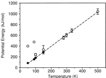
Fig. 3. Potential energy vs. temperature. The values of the

poten-Ž

tial energy of the initial configurations were discarded typically

.

t-300 ps in order to get equilibrium values. Open circles represent the values obtained for simulations which started with linear structures. Filled diamonds started with folded structures. The equilibrium values show a linear dependence on the tempera-ture.

reached that value. The other two values fluctuate around the equilibrium energy, although that repre-sented by filled circles shows more fluctuations. We assume that this occurs due to the fact that the initial

Ž .

configuration for Ts50 K is more folded than that expected for Ts150 K. So, the unfolding process presumably produces those fluctuations.

The increase of total average energy of the system is due to both kinetic and potential terms. Fig. 3 shows the values of the potential energy for all simulations. Open circles represent the simulation that started with a linear structure, while filled dia-monds represent those which started with a folded structure. As one can observe, for lower

tempera-Ž .

tures 50, 90, 100, 150 K the value of the potential energy is higher than that obtained for folded initial structure. Note that we used the data for the calcula-tions which were obtained after the system reached the equilibrium, i.e., where the energy fluctuates around a stable value. Typically, we discarded the initial 300 ps of simulations. The small error bars

Ž

obtained for the lowest temperatures 50, 90 and 100

.

K come from the fact that they are in a meta-stable state – as discussed above – and that the fluctuations in this case are small. Note that for Ts150 K the

Ž

potential energy for the case where the initial

struc-.

represent-ing the fact that the system has not stabilised. The dashed line in this figure represents a linear regres-sion made with the equilibrium values. Thus, we can assume that the equilibrium potential energy shows a linear dependence with the temperature for the com-plete temperature interval of our simulations.

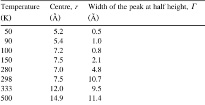
Table 1 shows the fitting of the end-to-end carbon distances to Gaussian functions, using the data ob-tained from equilibrium structures. We observe an

Ž .

increase of the width of the peak at half height G Ž .

and in the centre values r with increasing

tempera-Ž

ture. We related the end-to-end carbon distance less

.

folded structures and increasing conformational dis-tribution for PEO with the temperature increase. For higher temperatures, the width of the curve is of the order of the magnitude of its centre, while for lower temperatures this relation is around 30%. This means that for higher temperatures strong fluctuations are present.

In order to describe in more detail the equilibrium structures obtained in our simulations, we calculated the radius of gyration of the molecule for different temperatures. The radius of gyration R is given by_g

2 Ým Ri i

Rgs

)

,

Ž .

4

Ými

where m is the mass of the ith atom of the polymer,i

< <

Risriyrcm, r is the actual position of the ithi

atom and rcm is the centre of mass position of the polymer. Fig. 4 shows the results obtained for the equilibrium configurations. As one can observe, the higher the temperature is, the larger is the radius of

Table 1

Gaussian fitted parameters related to conformational population distribution curves as a function of end-to-end carbon distances over the temperature range 50–500 K

Temperature Centre, r Width of the peak at half height,G

˚ ˚

Ž .K Ž .A Ž .A

50 5.2 0.5

90 5.4 1.0

100 7.2 0.8

150 7.5 2.1

280 7.0 4.8

298 7.5 10.7

333 12.0 9.5

500 14.9 11.4

Fig. 4. Gyration radii of final configurations vs. temperature. The average was obtained taking into account the configurations at

ts500, 600, 700, 800, 900 and 1 000 ps. The data show a non-linear dependence with temperature. The inset figure shows the gyration radii behaviour when the temperature is decreased in the MD simulation.

Ž

gyration the increase of the radius of gyration is not

.

linear with temperature . Moreover, the fluctuations increase with temperature, the same phenomenon as observed for the end-to-end carbon distances. An interesting aspect that can be observed in Fig. 4 is the behaviour of the radius of gyration when a simulation is made by decreasing the temperature, where it is found that Rg decreases and remains

Table 2

Ž .

Thermodynamic properties in kcalrmol for the folding process in the PEO molecule

o a o b c o d

T DHT DST DZPE DGT Ž .K

e

100 y21.094 0.020 4.221 y18.873

f

100 y23.158 0.022 5.860 y19.498 298 y17.284 0.051 5.929 y26.553 500 y5.979 0.080 5.717 y40.262

a_DHo_sDHo _Žfolded.yDHo _{Žlinear , where the. DH}o _{is the}

T f, T f, T f, T

heat of formation calculated at the temperature T.

b_DSo_{sS folded}o_{Ž .yS linear .}o_{Ž .}

T T T

c_{D Ž . Ž .}

ZPEsZPE foldedyZPE linear . ZPE is the zero-point en-ergy.

d_D

Go_sDHo_yTDSo_qDZPE.

T T T

e

Structure obtained from the simulation started with linear geome-try.

f

Table 3

Ž .

Values of conformational energy terms E in kJrmol for PEO containing 20 monomeric units in a vacuum, CHCl and H O at3 2

298 K

Energy Evacuum ECHCl3 EH O2

ŽkJrmol. ŽkJrmol. ŽkJrmol.

kinetic 546 546 546

H stretching 191 190 193

bending 296 294 291

torsion 118 120 111

vdW y103 y63 y101

electrostatic 109 119 151

GvdWqGcav 0 y118 64

Gpol 0 y19 y171

a

total energy 1157 1067 1084

a

Standard deviation;2%.

practically constant. This means that folded struc-tures are definitely preferable to linear ones.

In the discussion presented previously, only the enthalpic contribution to the free energy has been considered for the folding process analysis. In order

Ž o_.

to analyse the entropy S change, the

semiempiri-w x o

cal AM1 method 12 was used to calculate the ST

values for the linear and folded structures at Ts100, 298 and 500 K. The folded equilibrium structures obtained from the MD simulations at the respective temperatures were used as starting points in the geometry optimisation procedure at the

semiempiri-cal level. The fully optimised geometries were used in the calculation of the thermodynamic properties. The results obtained are reported in Table 2. Analysing the values in Table 2, an increase of D_Ho

with T, can be seen showing that the folding process should be less favourable at higher temperature when only the energetic contribution to the free energy is considered. However, when the entropic contribution

Ž_DSo_{. is considered, the folding process was found} Ž

to be more favourable more negative values of

o_. o

D_{G as the temperature rises, the term yT}D_S being dominant at T)298 K.

Table 3 presents different contributions of the energetic terms obtained after simulations of the PEO in a vacuum, CHCl3 and H O. By analysing2

the intramolecular potential, it was noted that the principal changes due to the solvent were observed

Ž .

for the van der Waals vdW and electrostatic inter-action terms. Intermolecular contributions to the

sol-Ž .

vation process are present as GvdWqGcav and G .pol

Ž .

The results of the calculations for GvdWqGcav

showed an associated nature of the water because it needs an energy consumption to form cavities in the solvent. The G_pol term represents a solute–solvent electrostatic interaction energy, proportional to the dielectric constant of the medium. Fig. 5 shows the conformational population distribution as a function of end-to-end carbon distance. The end-to-end

car-Ž .

bon distance adjusted as described above shows an

average distance increase as a function of the medium in the following order: CHCl3)H O2 )vacuum. The structural effect described by the end-to-end carbon distance can be related to the degree of folding of the structure, considering that the principal energetic contribution in the macromolecules folding processes involves non-bonded atom interactions. The values obtained for the vdW terms can be used to justify the degree of folding observed in different media. These

Ž

values showed that EvdW has higher values more

.

repulsive for CHCl3 leading to less folded

struc-˚

Ž .

tures EvdWs y63 kJrmol and rs12.89 A . It can be seen that EvdWs y103 kJrmol in the absence of solvent and EvdWs y101 kJrmol in H O carrying2

to more folded structures, in agreement with the

Ž

centre distribution values shown in Fig. 5 rs7.45

˚

˚

.

A in a vacuum and rs9.70 A in H O .2

4. Conclusions

Mechanical and dynamic methods were applied in order to investigate the behaviour of PEO containing 20 monomeric units as a function of temperature and solvent. From the simulations performed in the tem-perature range of 50–500 K, we concluded that both kinetic and potential terms are responsible for the increase in the total energy as a function of tempera-ture. We have obtained folded final structures as the equilibrium structures for all temperatures. For lower temperatures, the system might be ‘trapped’ in a meta-stable state when the simulations were started with a linear structure. Besides, we could relate the

Ž .

end-to-end carbon distance less folded structures and conformational distribution variation for PEO with an increase in temperature. Moreover, we also observed that the radius of gyration increases with temperature, but it did not show a linear dependence on the temperature. It was also observed that the entropic contribution is important for the folding

< o_<

process at higher temperature, the term yTD_S

< o_<

being )D_{H at T)298 K.}

It was found that the behaviour of PEO in a vacuum, CHCl3 and H O is similar, where a ten-2

dency of PEO to assume a folded structure in the equilibrium was shown. The solvation energy results,

obtained using the GBrSA model, confirm this

ten-Ž

dency. The values in both solvents CHCl3 and

.

H O were found to be close and slightly less than in2

a vacuum. The structural effect observed in the analysis of the end-to-end carbon distance

equilib-Ž

rium structures average distance CHCl3)H O2 ) .

vacuum was related to the non-bonded atom interac-tions.

Acknowledgements

The authors would like to thank the Conselho

Ž .

Nacional de Desenvolvimento Cientıfico CNPq for

´

providing the research grants. Thanks are also due to

&

the Fundac

¸ao de Amparo a Pesquisa do Estado de

Ž .

Minas Gerais FAPEMIG and the Programa de Apoio ao Desenvolvimento Cientıfico e Tecnologico

´

´

ŽPADCT, Proc. No. 62.0241r95.0 for supporting.

this project. HFDS would like to thank the Nucleo de

´

Acesso Remoto-UFJF, CENAPAD-MGrCO, for the computational facilities.

References

w x1 V.N.R. Pillai, M. Mutter, Acc. Chem. Res. 14 1981 122.Ž .

w x2 A.D. Robertson, K.P. Murphy, Chem. Rev. 97 1997 1251.Ž .

w x3 N. Clinton, P. Matlock, Encyclopedia of Polymers, Vol. 6, John Wiley & Sons, New York, 1986, p. 225.

w x4 A. Apicela, B. Cappello, M.A. Del Nobile, M.I. La Rotonda, G. Mensitieri, L. Nicolais and S. Seccia, Polymeric Drugs and Drug Administration, Am. Chem. Soc., Washington, DC, 1994.

w x5 M. Armand, Solid State Ionics 69 1994 309.Ž .

w x6 K. Murata, Electrochim. Acta 40 13Ž . Ž1995 2177..

w x7 M. Armand, J.Y. Sanchez, M. Gauthier, Y. Choquette, in: J.

Ž .

Lipkowski, P.N. Ross Eds. , Electrochemistry of Novel Materials, ch. 2, VCH, New York, 1994.

w x8 W.L. Jorgensen, J. Tirado-Rives, J. Am. Chem. Soc. 110

Ž1988 1657..

w x9 F. Mohamadi, N.G.J. Richards, W.C. Guida, R. Liskamp, M. Lipton, C. Caufield, G. Chang, T. Hendrickson, W.C. Still, J.

Ž .

Comput. Chem. 11 1990 440.

w10 Special issue on Molecular Mechanics and Modelling, Chem.x

Ž .

Rev. 93 1993 .

w11 W.C. Still, A. Tempczyk, R.C. Hawley, T. Hendrickson, J.x

Ž .

Am. Chem. Soc. 112 1990 6127.

w12 M.J.S. Dewar, E.G. Zoebish, E.F. Healy, J.J.P. Stewart, J.x

Ž .