Integrated Georeferencing of LiDAR and Camera Data Acquired from a Moving Platform

INTEGRATED GEOREFERENCING OF LIDAR AND CAMERA DATA ACQUIRED

FROM A MOVING PLATFORM

F. Liebold, H.-G. Maas

Institute of Photogrammetry and Remote Sensing, Technische Universität Dresden, Germany frank.liebold@tu-dresden.de, hans-gerd.maas@tu-dresden.de

Commission III, ICWG III/I

KEY WORDS: laser scanning, bundle block adjustment, trajectory

ABSTRACT:

This paper presents an approach for modeling the trajectory of a moving platform equipped with a laser scanner and a camera. In most cases, GNSS and INS is used to determine the orientation of the platform, but sometimes it is impossible to use GNSS, especially indoor applications should be mentioned here. INS has a bad error propagation without GNSS. In addition, the accuracy of GNSS and low-cost INS is limited and often not equivalent to the accuracy potential of laser scanners. For the camera, there exists the well-known alternative to obtain the orientation parameters via triangulation, for instance employing structure-from-motion techniques. But it is more challenging to find an alternative for the laser scanner, because of its sequential data acquisition. In the approach shown here, we propose to use a camera in combination with structure-from-motion techniques as the basis for determining the laser scanner trajectory parameters. For that purpose, we use piece-wise models for the trajectory through polynomial functions, supported by time-stamped matches between laser scanner and camera data.

1. INTRODUCTION

Cameras and laser scanners are tools for spatial data acquisition. If they are used on moving platforms such as UAVs or robots, it is essential to know their position and orientation parameters during the scanning process. GNSS and INS are often used for the determination of the pose of the laser scanner. In certain applications, however, it may be impossible to use GNSS and/or it may be beneficial to work without INS, for instance due to adverse error propagation. Camera orientation parameters can be determined by well-known aero-triangulation techniques or by structure-from-motion tools, if there is enough overlap between the images. For the laser scanner it is more difficult to find an adequate alternative, mainly due to its non-redundant sequential data acquisition nature. Furthermore, the accuracy of a laser scanner is often superior to GNSS accuracy, leading to the accuracy potential being deteriorated in the georeferencing process especially when light-weight low-cost GNSS components are being used. The main goal of the approach presented here is to obtain a trajectory (time-resolved 6-dof pose data) for the laser scanner with a higher accuracy based on matching features between image and laser scanner data. Thus, structure-from-motion techniques applied to high resolution camera image sequences from the base for trajectory determination. Doing so, we have to cope with the different temporal resolution of camera and laser scanner. This is in first instance considered by a cubic polynomial as mathematic model for the trajectory piece between two images of the camera, with the polynomial parameters obtained from the photogrammetric image sequence processing and the laser scanning data.

(Zhang et. al., 2013) present a related method. They propose a LiDAR strip adjustment method which is aided by GPS and INS. At first an aero-triangulation with ground control points is conducted in their approach, subsequently the areal images are

matched with generated LiDAR intensity images using Harris corners. They use quadratic polynomials for X, Y, Z (point of origin of the laser scanner) and omega, phi, kappa (rotation parameters of the laser scanner).

In our approach, cubic polynomials are used for each extrinsic parameter of the the laser scanner and the rotations are modeled with quaternions. Furthermore, we try to include the matching results between image and laser scanner data as observations in an integrated bundle adjustment.

In the piece-wise polynomial model for the trajectory section between two time instances ti and ti+1 the position of origin of the laser scanner is expressed:

XL

0₍

t) = XL

0₍

ti)+si11⋅(t ti)+si12⋅(t ti)

2₊

si13⋅(t ti)

3

YL

0₍

t) = YL

0₍

ti)+si21⋅(t ti)+si22⋅(t ti)

2₊

si23⋅(t ti)

3

ZL

0

(t) = ZL

0

(ti)+si31⋅(t ti)+si32⋅(t ti)

2

+si33⋅(t ti)

3 (1)

Quaternions of laser scanner orientation:

aL'(t) = aL(ti)+si41⋅(t ti)+si42⋅(t ti)

2₊

si43⋅(t ti)

3

bL'(t) = bL(ti)+si51⋅(t ti)+si52⋅(t ti)

2₊

si53⋅(t ti)

3

cL'(t) = cL(ti)+si61⋅(t ti)+si62⋅(t ti)

2

+si63⋅(t ti)

3

dL'(t) = dL(ti)+si71⋅(t ti)+si72⋅(t ti)

2₊

si73⋅(t ti)

3

(2)

The interpolated quaternions have to be normalized:

n=(aL'(t)

2₊

bL'(t)

2₊

cL'(t)

2₊

dL'(t)

2₎0.5

aL(t)=aL'(t)⋅n bL(t)=bL'(t)⋅n

cL(t)=cL'(t)⋅n dL(t)=dL'(t)⋅n

(3) The International Archives of the Photogrammetry, Remote Sensing and Spatial Information Sciences, Volume XL-3, 2014

where X0L(t), Y0L(t), Z0L(t) = coordinates of the point of origin of the laser scanner at time t

i = index over images

j = index over extrinsic parameters

k = index over degree of the polynomial

sijk = polynomial parameters

ti = acquisition time of the last image with index i

a'L(t), b'L(t), c'L(t), d'L(t) = not normalized quaternions of the laser scanner orientation at time t

aL(t), bL(t), cL(t), dL(t) = quaternions of the laser scanner orientation at time t

The paper is organized as follows: Section 2 describes the workflow how to acquire the trajectory. The following sections go into detail of some single steps from the overall workflow. The last section gives a conclusion and outlook.

2. WORKFLOW

A typical dataset to be processed consists of images and laser scanner measurements taken from a moving platform. The images will usually have a time interval of about a second, if they are taken by high resolution light-weight camera, while the laser scanner will have a data rate in order of 50-200 kHz. Low precision GNSS and INS data may be available and used as approximate values, but is not a pre-requisite. Some control points should be available for datum definition. The data processing chain can be sketched like this (see also Figure 1):

1) Beforehand, the intrinsic parameters of the camera are determined by self calibration; as an alternative, the camera parameters may also be determined by simultaneous calibration.

2) The next preparation step is the determination of the relative orientation between laser scanner and camera (platform calibration, bore-sight alignment). This can be done by scanning objects of known geometry such as cones as described in (Mader et. al., 2014). 3) The actual data acquisition takes images and laser

scanner measurements along a trajectory of a UAV or some robot.

4) Then the orientation parameters of all images determined using a structure-from-motion tool. 5) The laser scanner orientation parameters at the image

acquisition time steps can be computed using the parameters of the relative orientation.

6) A computation of adapted cubic splines for the laser scanner orientation parameters provides initial values for the polynomial parameters.

7) With the aid of the (initial) trajectory of the laser scanner a point cloud is generated from the laser scanner data.

8) Intensity images are computed by projecting the point cloud from the laser scanner data in virtual images. These images are the basis for matching between the image and laser scanner data.

9) The next step is a matching between the camera images and the laser scanning data. In our approach it is based on descriptor matching techniques (intensity image from the laser scanner data and the camera

image) to get homologous features extracted from both data.

10) Then follows the central step of an integrated bundle adjustment with the LiDAR and image data with the time-stamped homologous points between laser scanner and image data as observations and the trajectory parameters introduced as unknowns. 11) In an additional step, an adaptive balancing of the

standard deviations of the different groups of observations can be done in order to improve the stochastic model (variance component estimation). 12) Then the computed polynomial parameters from the

bundle adjustment are used as new initial values and the steps 7 to 12 are repeated until it is converged. 13) Finally, all laser scanner measurements can be

converted into XYZ coordinates using the trajectory parameters and the time-stamped laser scanner range measurements.

Some of these steps are explained in more detail later.

Figure 1. Data processing chain

3. PLATFORM CALIBRATION

As a pre-requisite for further data processing, the system components should be calibrated. This can either be performed a priori, as outlined in this section, or through simultaneous calibration during the actual data processing (section 5).

The platform calibration includes the determination of the six fix parameters of the relative orientation between camera and scanner. As described in (Mader et. al., 2014) cones are used to realize this. The orientation of the laser scanner can be The International Archives of the Photogrammetry, Remote Sensing and Spatial Information Sciences, Volume XL-3, 2014

computed by minimizing the distances of the laser scanner points to the surface of the cones. The geometry of the cones is determined in the course of an extended photogrammetric bundle adjustment. The extrinsic parameters are considered as unknowns in the least squares problem, requiring at least 3 cones. Figure 2 shows the calibration environment.

Figure 2. Calibration environment

The results of such a calibration are shown in Table 1.

Value Standard deviation

point of origin: X0 [mm] Y0 [mm] Z0 [mm]

quaternions: a [-] b [-] c [-] d [-] 372.285 -23.671 47.400 0.69343 0.23252 0.24956 -0.63467 0.48 1.86 0.42 0.00063 0.00051 0.00055 0.00067

Table 1. Results of the platform calibration: the extrinsic parameters of the laser scanner in the camera coordinate system

4. DATA AQUISITION AND TRIANGULATION OF THE IMAGES

For test purposes, we used a platform equipped with an industrial CCD camera (AVT Prosilica GT 3300C) and a light-weight 2D laser scanner (Hokuyo UTM-30LX). The data was acquired after the calibration process. It is crucial to record time stamps for the camera images and laser scanning measurements in the same time system to assign the data. The first step of the following data analysis is the image triangulation, which can be realized with the VisualSFM software (Wu, 2011). The corresponding image points derived from VisualSFM are improved with Least Squares Matching (Gruen, 1985), followed by a new bundle adjustment with the improved image coordinates. We use the SfM_georef software (James et. al., 2012) to get the output to scale. As result, the true scaled orientation parameters of the images are obtained.

In a next step, the orientation parameters of the laser scanner for the image acquisition time instances are computed with the aid of the relative orientation given from the calibration procedure.

5. INITIAL VALUES FOR THE POLYNOMIAL PARAMETERS

The integrated bundle adjustment for the determination of the time-resolved trajectory parameters requires initial values. These initial values for the polynomial parameters can be determined by computing a spline. Control points for this spline are the orientation parameters of the laser scanner for the image acquisition time instances (derived from the extrinsic parameters of the camera images and the relative orientation from section 3) through the whole trajectory.

The spline function sX for the extrinsic parameter X of the laser scanner orientation according to the image i is:

s_ix

(t₎₌a_i⋅(t t_i)3

+b_i⋅(t t_i)2

+c_i⋅(t t_i)+x_i

0.5⋅(ti 1+ti)<t<0.5⋅(ti+ti+1)

(4)

where i = 1..n index over the function values n = number of given function values ai, bi, ci = unknowns spline parameters t = time variable

ti = time for the function value i t0 = t1 and tn+1 = tn

xi = x coordinate with index i = function value i

Some constraints are defined.

The spline should form a continuous function:

s i x

(0.5⋅(t

i+ti+1))=si+1 x

(0.5⋅(t

i+ti+1)) (5)

The first derivative should be continuous:

∂

s

∂

t

|

i+ti+1)

=

∂

s

∂

t

|

(6)

The second derivative should be continuous:

∂2

s i x

∂t2

|

=∂

2

s i+1

x

∂t2

|

(6)

Thus, 3·n-3 constraints can be derived, but there are 3·n unknowns. For this reason, 3 other constraints are necessary, for instance:

b

=

b

=

c

=

0

Now a linear system of equations can be set up and solved. The splines for Y, Z and for the quaternions can be computed in the same way.

Figure 4 shows the trajectory of laser scanner. The blue points are the interpolated points of origin of the laser scanner computed with the aid of the spline parameters. The camera orientations are visualized as green pyramids. The base lines between the point of origin of the laser scanner and the projection center of the camera at the acquisition time instances of the images are displayed as cyan lines. The axes of the laser scanner coordinate system at the acquisition time of the images are visualized as well (X-axis: red; Y-axis: green; z-axis: blue). The International Archives of the Photogrammetry, Remote Sensing and Spatial Information Sciences, Volume XL-3, 2014

Figure 4. Initial trajectory by spline computation

6. MATCHING

Having computed the spline parameters for the orientation parameters, a first point cloud can be generated from the laser scanner data using the initial trajectory of the laser scanner and its distance measurements. Note that this initial point cloud will be sub-optimal, due to the relatively long time interval between the image capture time instances and the irregular movement of the platform. The central goal of the approach is to refine this trajectory using tie points between the images and the laser scanner point cloud.

To obtain these tie points, a matching between the LiDAR and the image data is performed. Different approaches have been used for LiDAR and image data registration, for instance the feature-based image matching method SIFT (Lowe, 2004), a frequency-based LPFFT (log-polar fast fourier transformation) or the intensity-based mutual information technique. These methods are described and compared in (Ju et. al., 2012). They also present a new approach, which combines these techniques to take advantage of all of them and make it more robust. (Meierhold et. al., 2010) also presents a method for automatic feature matching between digital images and 2D representations of 3D Laser scanner point clouds based on SIFT descriptor matching.

In the approach presented here, we combine the FAST Feature detector and SIFT descriptor matching to find matches between the image data and an intensity image generated from the laser scanner point cloud.

The projection centers of the intensity images are placed into the points of origin of the laser scanner at the acquisition time steps of the corresponding camera images. The rotation matrices are set to those of the corresponding camera image.

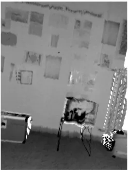
An example of such an intensity image is shown in figure 5. Herein, the degradations caused by the preliminary trajectory deficits as described above are obvious.

For the matching process between the camera images and the intensity images derived from the laser scanner data, it turned out to be sometimes necessary to scale the images because to prevent artifacts of scaling invariant feature detectors. The image of the camera is scaled so that the dimensions of the camera image and the intensity image are approximately identical. The FAST feature detector is applied to both images, and for all interest points a SIFT descriptor is computed. Now the 3D coordinates of the feature points in the intensity image are determined. To realize this, the nearest neighbors to the feature points in the projected laser scanner points are obtained. Subsequently the average of the 3D points is computed. These 3D points can be projected into the camera image. These image points should be approximately the homologous points in the camera image.

Now the descriptor distances are computed for the nearest neighbors within a given radius to this image point. A first result is shown in figure 6, the corresponding points are connected. There are still some small errors, which are mainly caused by the different characteristics of the intensity image and the camera image.

Figure 5. Intensity image

7. INTEGRATED BUNDLE ADJUSTMENT

The integration of LiDAR and image data in a bundle adjustment and a variance component estimation has been shown in (Schneider et. al., 2007). The approach here is similar. In addition to the observations of the laser scanner there are some more unknowns for the trajectory parameters now.

The following variables are introduced as unknowns: • the parameters for the time-resolved trajectory • the 3D coordinates of the corresponding points • optionally the extrinsic parameters of the camera

images

• optionally the intrinsic parameters of the camera • optionally the parameters for the relative orientation

between camera and laser scanner

The observations are listed here:

• image coordinates of the tie points in the camera images

• the laser scanner measurements for the tie points • optionally some object distances to improve the scale

There are some constraints, too:

• constraints for quaternions of the camera orientations (sum of squares is equal to one)

• optionally some constraints for the free network adjustment

• optionally constraints for the trajectory parameters, for instance continuous function values of the polynomials

It is crucial, that all observations, especially the laser scanner measurements, are introduced with a time-stamp to warrant proper relation to the time-resolved trajectory.

Figure 6. Matching result, the corresponding points are connected

The bundle adjustment is iterative. The improved parameters are considered as new initial values. Using these parameters, a new (improved) 3D point cloud and new intensity images can be computed from the laser scanner data, which are then again fed into the image-scanner matching routine. These steps are repeated until the process converges.

An adaptive balancing of the standard deviations of the observations can be performed in an additional step to improve the stochastic model.

At this stage, no results of the integrated bundle adjustment can be shown, as this is ongoing work.

8. CONCLUSION AND OUTLOOK

This paper presented a method to achieve time-resolved trajectory parameters for a moving platform. First partial results have been shown, proving the possibility of using an image-based trajectory for generating a preliminary 3D point cloud from laser scanner data and the feasibility of matching between images and laser scanner data. The main steps, that have to be done in the future, are the integrated bundle adjustment and the variance component estimation. Furthermore, there is potential to improve the matching.

ACKNOWLEDGEMENTS

The research work presented in this paper has been funded by the German Research Council (DFG).

REFERENCES

Gruen, A., 1985. Adaptive least squares correlation – a powerful image matching technique. South African Journal of Photogrammetry, Remote Sensing and Cartography, 14(3), pp. 175-187.

James, M., Robson, S., 2012. Straightforward reconstruction of 3D surfaces and topography with a camera: Accuracy and geoscience application. J. Geophysical Res., 117, F03017

Ju, H., Toth, C., Grejner-Brzezinska, D., 2012. A New Approach to Robust LiDAR/Optical Imagery Registration. Photogrammetrie-Fernerkundung-Geoinformation, Volume 2012, Number 5, October 2012, pp. 523-534.

Lowe, D., 2004. Distinctive Image Features from Scale-Invariant Keypoints. International Journal of Computer Vision, 60(2), pp. 91-110.

Mader, D., Westfeld, P., Maas, H.-G., 2014. An Integrated Flexible Self-calibration Approach for 2D Laser Scanning Range Finders Applied to the Hokuyo UTM-30LX-EW. In: The International Archives of Photogrammetry, Remote Sensing and Spatial Information Sciences, Volume XL-5,2014, pp. 385-393.

Meierhold, N., Spehr, M., Schilling, A., Gumhold, S., Maas, H.-G., 2010,Automatic feature matching between digital images and 2D representations of a 3D laser scanner point cloud. In: TheInternational Archives of Photogrammetry, Remote Sensing and Spatial Information Sciences, Vol. 38, Part 5, WG V/3.

Rosten, E., Drummond, T., 2005. Fusing points and lines for high performance tracking. Proc. 10th IEEE International Conference on Computer Vision (ICCV'05), Volume 2, Beijing, pp. 1508-1515.

Schneider, D., Maas, H.-G., 2007. Integrated bundle adjustment of terrestrial laser scanner data and image data with variance component estimation. The Photogrammetric Journal of Finland, Volume 20/2007, pp. 5-15.

Wu, C., 2011. VisualSFM: A Visual Structure from Motion System. http://ccwu.me/vsfm/ (25.07.14)

Zhang, Y., Xiong X., Hu, X., 2013. Rigorous LiDAR Strip Adjustment with Triangulated Aerial Imagery. ISPRS Annals of Photogrammetry, Remote Sensing and Spatial Information Sciences, Volume II-5/W2, 2013, pp. 361-366.