www.atmos-chem-phys.net/12/3837/2012/ doi:10.5194/acp-12-3837-2012
© Author(s) 2012. CC Attribution 3.0 License.
Chemistry
and Physics
Evaluating the influences of biomass burning during 2006
BASE-ASIA: a regional chemical transport modeling
J. S. Fu1, N. C. Hsu2, Y. Gao1, K. Huang1, C. Li2,3, N.-H. Lin4, and S.-C. Tsay2
1Department of Civil and Environmental Engineering, University of Tennessee, Knoxville, TN, USA 2NASA/Goddard Space Flight Center, Greenbelt, MD, USA
3Earth System Science Interdisciplinary Center, University of Maryland, College Park, MD, USA 4Department of Atmospheric Sciences, National Central University, Chung-Li, Taiwan
Correspondence to:J. S. Fu (jsfu@utk.edu)
Received: 9 September 2011 – Published in Atmos. Chem. Phys. Discuss.: 7 December 2011 Revised: 5 March 2012 – Accepted: 8 April 2012 – Published: 2 May 2012
Abstract. To evaluate the impact of biomass burning from Southeast Asia to East Asia, this study conducted nu-merical simulations during NASA’s 2006 Biomass-burning Aerosols in South-East Asia: Smoke Impact Assessment (BASE-ASIA). Two typical episode periods (27–28 March and 13–14 April) were examined. Two emission inventories, FLAMBE and GFED, were used in the simulations. The in-fluences during two episodes in the source region (Southeast Asia) contributed to the surface CO, O3and PM2.5
concen-trations as high as 400 ppbv, 20 ppbv and 80 µg m−3,
respec-tively. The perturbations with and without biomass burning of the above three species during the intense episodes were in the range of 10 to 60 %, 10 to 20 % and 30 to 70 %, re-spectively. The impact due to long-range transport could spread over the southeastern parts of East Asia and could reach about 160 to 360 ppbv, 8 to 18 ppbv and 8 to 64 µg m−3 on CO, O3 and PM2.5, respectively; the percentage impact
could reach 20 to 50 % on CO, 10 to 30 % on O3, and as high
as 70 % on PM2.5. In March, the impact of biomass burning
mainly concentrated in Southeast Asia and southern China, while in April the impact becomes slightly broader and even could go up to the Yangtze River Delta region.
Two cross-sections at 15◦N and 20◦N were used to com-pare the vertical flux of biomass burning. In the source re-gion (Southeast Asia), CO, O3and PM2.5concentrations had
a strong upward transport from surface to high altitudes. The eastward transport becomes strong from 2 to 8 km in the free troposphere. The subsidence process during the long-range transport contributed 60 to 70 %, 20 to 50 %, and 80 % on CO, O3and PM2.5, respectively to surface in the downwind
area. The study reveals the significant impact of Southeast-ern Asia biomass burning on the air quality in both local and downwind areas, particularly during biomass burning episodes. This modeling study might provide constraints of lower limit. An additional study is underway for an active biomass burning year to obtain an upper limit and climate ef-fects.
1 Introduction
strong evidence that both natural and anthropogenic biomass burning constitute a major component in land-atmosphere carbon flux anomalies. Potter et al. (2001) reported the es-timation of carbon losses by biomass burning on the Brazil-ian AmazonBrazil-ian region from ecosystem modeling and satellite data analysis.
Although biomass burning studies in the last decade have focused on the physical, chemical, and thermodynamic prop-erties of biomass-burning particles (Reid et al., 2005), model simulation results of biomass burning aerosol are still lim-ited. Most of recent model studies focus on Mexico, South America and Africa, like several recent field projects includ-ing SAFARI 2000 (Swap et al., 2003), LAB-SMOCC (Chand et al., 2006; Guyon et al., 2005), the Dust and Biomass-burning Experiment (Haywood et al., 2008) and African Monsoon Multidisciplinary Analysis (Mari et al., 2008).
Southeast Asia is one of the major biomass-burning emis-sion source regions in the world (Streets et al., 2004). Both biomass and fossil combustion processes are potential sources of the extensive Asian Brown Clouds (ABC) over South Asia (Gustafsson et al., 2009). The smoke plume from biomass burning generally spreads downwind thousands of kilometers away and affects air quality, human health, and regional climate. To date, information on the regional distri-bution of biomass-burning aerosols from Asia remains lim-ited, and their regional radiative impact is not well under-stood (Wang et al., 2007).
Early studies showed the springtime high ozone events in the lower troposphere from Southeast Asian biomass burn-ing (Liu et al., 1999). The effects of Southeast Asia biomass burning on aerosols and ozone concentrations over the Pearl River Delta (PRD) region was studied using satellite data, ground measurements, and models; it was suggested that O3
productivity is reduced due to the reduced UV intensity under the influence of Southeast Asia biomass burning (Deng et al., 2008). Choi and Chang (2006) described the use of MOPITT to evaluate the influence of Siberian biomass burning on CO levels around Korea and Japan. Spatial distributions of black carbon (BC) and organic carbon (OC) aerosols were simu-lated along with the radiative forcing of the Asian biomass burning (Wang et al., 2007). The influence of biomass burn-ing from Southeast Asia on CO, O3and radical (OH, HO2)
outflow was also simulated by Tang et al. (2003). A new transport mechanism of biomass burning from Indochina was discovered using the WRF/Chem model (Lin et al., 2009). Despite these efforts, however, comprehensive estimates of the impact of Southeast Asia biomass burning on the down-stream regions are still lacking.
This study is part of NASA’s BASE-ASIA experiment (Biomass-burning Aerosols in South-East Asia: Smoke Im-pact Assessment; cf. http://smartlabs.gsfc.nasa.gov/) in 2006. One of the objectives of BASE-ASIA is to investi-gate the regional impact of biomass burning on Southeast and East Asia. Besides the air quality impact resulting from biomass burning, the biomass burning aerosols could also
af-fect radiative forcing. However, large uncertainty exists in coupled climate/air quality models, especially aerosol feed-back may not be fully implemented (Zhang, 2008) and in the estimates of emission inventories, this study identifies the influences of biomass burning on East Asia during in-tense burning episodes by employing a regional “one atmo-sphere” model, the Community Multiscale Air Quality Mod-eling System (CMAQ) (Byun and Schere, 2006; Byun and Ching, 1999) in the offline mode. Model simulations were compared with satellite observations and in situ ground mea-surements to validate the model. Two different biomass burn-ing emission inventories were evaluated. Model simulations were compared with satellite observations and in situ ground measurements to validate the model, including PM2.5, trace
gases and aerosol optical depths. The long-range transport and vertical transport patterns of particles and trace gases were illustrated and quantified by conducting scenario simu-lation of cutting off the biomass burning emission.
2 Methodology
2.1 Model description
Table 1.Model configuration of WRF and CMAQ.
WRF Configuration
Meteorology model WRF v3.1.1
Explicit precipitation scheme WRF single – moment 3 – class scheme
Longwave Radiation RRTM
Shortwave Radiation Dudhia scheme
Surface-layer option MM5 similarity (Monin – Obukhov scheme)
Land-surface Thermal diffusion scheme
Advection Global mass-conserving scheme
Planetary boundary layer scheme YSU
Cumulus option Grell
CMAQ Configuration
Chemistry model CMAQ v4.6
Horizontal resolution 27×27 km
Vertical resolution 19 sigma-pressure levels (with the top pressure of 100 mb)
Projection Lambert Conformal Conic
Advection Piecewise parabolic scheme
Vertical diffusion K-theory
Gas-phase chemistry CB05 with Euler Backward Iterative solver (Hertel et al., 1993)
Dry deposition Wesely (1989)
Wet deposition Henry’s law
Aqueous chemistry Walcek and Aleksic (1998)
Aerosol mechanism AERO4
Fig. 1. The 27×27 km nested domain from the mother domain with a resolution of 81×81 km. Five countries with dominant biomass
burning emission in Southeast Asia in this study are colored (Pink: Burma; Bule: Thailand; Yellow: Cambodia; Red: Laos; Green: Vietnam). The observational sites used in this study for model performance are also plotted in the figure, including one site in Thailand (Phimai), four sites in Hong Kong (Tsuen Wan, Yuen Long, Tap Mun and Tung Chung) and one site in Taiwan (Hengchun).
2.2 Emissions
2.2.1 Anthropogenic emissions
Anthropogenic emissions are based on NASA’s 2006 In-tercontinental Chemical Transport Experiment-Phase B (INTEX-B) emission inventory (Zhang et al., 2009). The inventory mainly includes gaseous pollutants, such as CO2,
SO2, NOx, CO, CH4, and NH3; non-methane volatile organic
compounds (NMVOC); and particulate pollutants, such as submicron black carbon aerosol (BC), submicron organic carbon aerosol (OC), PM2.5, and PM10. NMVOC can be
cattle, pigs, other animals, fertilizer use, biofuel use, and other sources. The CH4 emissions were derived from rice
cultivation, animal emissions, landfill, wastewater treatment, coal mining/combustion, oil/gas extraction and use, and bio-fuel combustion (Du, 2008).
2.2.2 Biogenic and biomass burning emissions
Biogenic isoprene emissions were generated from MEGAN (Model of Emissions of Gases and Aerosols from Nature) to estimate regional and global biogenic emissions. In this study, MEGAN v2.02 was used to generate the hourly bio-genic emissions inventories (http://bai.acd.ucar.edu/Megan/ index.shtml).
The joint Navy, NASA, NOAA, and universities Fire Locating and Modeling of Burning Emissions (FLAMBE) project was used to investigate a consistent system of emis-sions (Reid et al., 2009). Hourly emisemis-sions from FLAMBE were taken from the 2006 data (http://www.nrlmry.navy.mil/ aerosol web/arctas flambe/data hourly/). The fire locations and emissions were computed based on the Global Land Cover Characterization Version 2 database (http://edc2.usgs. gov/glcc/glcc.php). This dataset contains hourly biomass burning of areas as well as carbon emissions in a certain lo-cation with coordinated latitudes and longitudes.
The Global Fire Emissions Database, Version 2 (GFEDv2.1), another biomass burning emission data source, is derived from MODIS fire count data (van der Werf et al., 2006). This dataset comprises eight-day periods throughout 2006 and monthly average emissions. In this study, carbon emissions from FLAMBE and GFED were both allocated to the simulation domain with a resolution of 27×27 km. Since the temporal resolution of GFED data is eight days, the hourly profile in FLAMBE was used to dis-tribute GFED emissions. Quantitative comparisons between the FLAMBE and GFEDv2.1 biomass emission inventories were conducted in this study before one inventory was selected to further estimate the regional impact of Southeast Asian biomass burning.
Both biomass burning emission inventories estimate carbon emissions, which were then converted to other species. Andreae and Merlet (2001) reported emission fac-tors (EF) for conversion from carbon emissions to other species (CO, CH4, NMHC, NOx, NH3, SO2, PM2.5,
TPM, OC and BC) in terms of different land use types, such as tropical forest, extratropical forest, agricultural residues, and savanna and grassland. Based on the 24 land use types (http://www.mmm.ucar.edu/wrf/users/docs/ user guide V3/users guide chap3.htm# Land Use and) and the WRF Preprocessing System (WPS) output, we catego-rized the land use types into several groups: EF of the grids with land use category 2, 3, 4 (Dryland Cropland and Pasture, Irrigated Cropland and Pasture, and Mixed Dryland/Irrigated Cropland and Pasture, respectively) were assigned to agri-cultural residues; EF of the grids with land use category 5, 6,
7, 8, 9, 10 (Cropland/Grassland Mosaic, Cropland/Woodland Mosaic, Grassland, Shrubland, Mixed Shrubland/Grassland, Savanna, respectively) were assigned to savannas and grass-lands; EF of the grids with land use category 11, 12, 14, 15 (Deciduous Broadleaf Forest, Deciduous Needleleaf Forest, Evergreen Needleleaf, and Mixed Forest, respectively) were assigned to extratropical forests; and the grids with land use category 13 (Evergreen Broadleaf) were assigned to tropical forests. Grids with other land use types usually do not have biomass burnings (van der Werf et al., 2006).
2.3 Injection height of biomass burning emission
Determining the injection height is important for the regional chemical model and could significantly affect long-range transport. Leung et al. (2007) used the GEOS-Chem global model to simulate the transport of boreal forest fire smoke under different scenarios and found different CO responses for different injection heights. Freitas et al. (2006) used the 1-D plume rise model to simulate the injection height of fire emissions and found that model outputs were more consistent when the injection height of vigorous fire reached mid-troposphere. Hyer et al. (2007) examined the injec-tion height under five different scenarios using the Univer-sity of Maryland CTM (Allen et al., 1996a, b) and found that pressure-weighted injection through the tropospheric column into the midtroposphere agreed the best with observations. In this study, we adopted the methodology implemented in Sparse Matrix Operator Kernel Emissions (SMOKE) ver-sion 2.6 for calculating the plume fractions in different layer heights given a bottom (Pbot) and top (Ptop) of a plume. The
hourly top of the plume was calculated as follows:Ptophour =
(BEhour)2·(BEsize)2·Ptopmax, where BE is the buoyant
ef-ficiency looked up from the hourly or size class tables. The hourly bottom of plume was similarly calculated as:Pbothour
= (BEhour)2·(BEsize)2·Pbotmax. The look up table of BEhour
and BEsizeare described by Air Sciences, Inc. (2005).
3 In-situ and satellite observation
3.1 BASE-ASIA field campaign
in detail elsewhere (Li et al., 2010) and is only briefly intro-duced here. CO was measured with a modified Thermo En-vironmental Instruments (Franklin, MA) Model 48C detector (Dickerson and Delany, 1988). A TEI Model 49C was used to monitor O3. Before and after, as well as every 3–4 weeks
during the field campaign, the CO instrument was calibrated with a working standard gas (Scott-Marrin Inc., Riverside, CA) traceable to National Institute of Standards and Tech-nology standard reference materials. The O3 detector was
calibrated with an in-house primary standard (TEI Model 49 PS). Aerosol size distribution was determined with an Aero-dynamic Particle Sizer spectrometer (APS, TSI Model 3321) and a Scanning Mobility Particle Sizer (SMPS, TSI Model 3081).
3.2 Observational sites in downwind regions
The Hengchun observation site in Taiwan is included in the Taiwan Air Quality Monitoring Network (TAQMN) operated by the Environmental Protection Administration. This is a background site located in the most southern part of Taiwan (102.77◦E, 21.95◦N) and is an ideal site for the observation of long-range transport of biomass burning from Southeast Asia. Continuous operations of hourly aerosol concentra-tion, trace gases, atmospheric radiaconcentra-tion, and meteorological variables are measured at this site. CO was measured by HORIBA/APMA-360, with a detection limit of 50 ppb; O3
was measured by ECOTECH/EC9810, with a detection limit of 0.5 ppb; and PM2.5was measured by Thermo/R&P 1400a
with a detection limit of 0.5 µg m−3.
Four sites in the Hong Kong Environmental Protection De-partment (HKEPD) Air Pollution Index (API) network are also used as observational stations for model evaluations. Two of them are Tsuen Wan and Yuen Long on the south-west and northsouth-west of Hong Kong, while the other two are Tap Mun and Tung Chung, which are remote sites located in the northeast of Hong Kong and Lantau Island. CO, O3, and
PM2.5were continuously measured during the study period.
Other detailed information was described elsewhere (Kwok et al., 2010).
3.3 Satellite observation
A number of satellite sensors launched in the past decade have proven valuable for studying anthropogenic pollution in the troposphere (Martin, 2008; Richter et al., 2005). In this study, we use the tropospheric NO2 product from the
Ozone Monitoring Instrument (OMI) aboard NASA’s EOS Aura satellite (for details of the OMI instrument and NO2
product, see Levelt et al., 2006 and Bucsela et al., 2006), and aerosol optical depth (AOD) retrieved from the MODer-ate Resolution Imaging Spectrometer (MODIS) instrument aboard the Aqua satellite (Krotkov et al., 2008) MODIS pro-vides remotely sensed aerosol information with a resolu-tion of 10×10 km for this study. Detailed information on
MODIS sensors and global daily observations of aerosols were used to retrieve aerosol properties over land (Remer et al., 2005) and ocean (Tanr´e et al., 1997). In this study, we use level 2 collection and 5 aerosol optical thickness at 550 nm. Both OMI NO2and MODIS AOD products have been widely
used in air quality studies to track regional aerosol plumes (Li et al., 2010a) and characterize power plant emissions (Li et al., 2010c).
4 Results and discussion
4.1 Comparison between FLAMBE and GFED emission inventory
Table 2. The monthly carbon emission (Tg) from GFED and FLAMBE biomass burning emission inventories in both Southeast Asia and outside Southeast Asia in the domain (Referred as East Asia) in 2006, respectively.
Carbon Southeast Asia East Asia
Emission GFED1 FLAMBE1 FLAMBE/GFED2 GFED1 FLAMBE1 FLAMBE/GFED2
Jan 5.54 14.01 2.53 0.4 4.97 12.39
Feb 8.06 35.79 4.44 1.16 10.13 8.73
Mar 28 220.9 7.89 18.24 84.79 4.65
Apr 13.43 156.22 11.63 1.58 21.13 13.39
May 0.9 8.74 9.7 1.78 6.08 3.42
Jun 0.21 1.39 6.72 1.24 1.25 1.01
Jul 0.03 0.12 3.81 0.94 0.66 0.7
Aug 0.02 0.08 3.54 1.36 1.09 0.8
Sep 0.1 0.23 2.3 0.44 0.92 2.09
Oct 0.12 0.47 4.02 0.73 2.21 3.02
Nov 0.55 1.92 3.47 0.59 3.31 5.65
Dec 2.08 7.6 3.66 0.33 3.27 9.97
Total 59.04 447.47 7.58 28.79 139.81 4.86
1The monthly carbon emission of GFED and FLAMBE are in units of Tg. 2The ratio of FLAMBE versus GFED (unitless).
Fig. 2.Model Performance of the temporal CO concentrations with
two different biomass burning emission inventories during 1 April to 31 May 2006 at Phimai, Thailand. The red line represents the ob-servation data, and the blue and purple lines represent the modeled CO concentration by using the FLAMBE and GFEDv2.1 biomass burning emissions, respectively.
April. While the simulation based on GFED emissions obvi-ously underestimated the CO concentrations during the peak periods by as much as 200 to 300 ppbv. This comparison indicated that the FLAMBE emission provided a better rep-resentation of biomass burning sources in our model than did the GFED emission. Nam et al. (2010) also found underes-timation of CO emissions at lower subtropical latitudes over Asia using the GFED emissions. Thus, in the further dis-cussion, we use the FLAMBE emission for sensitivity tests and analysis of the large-scale impact of biomass burning in Southeast Asia.
4.2 Model results and comparison with measurements
4.2.1 Comparison of simulations with site measurements
Figure 3 shows the model performance at ground-based sites in Taiwan and Hong Kong. Time-series of hourly CO, O3,
and PM2.5concentrations were evaluated. As shown in the
figure, the model successfully captured the temporal varia-tion at all sites during the whole study period, indicating relatively good model performance at the downwind sites. Some statistical parameters were used for model evaluations, including MNB (Mean Normalized Bias), MNE (Mean Nor-malized Gross Error), MFB (Mean Fractional Bias) and MFE (Mean Fractional Gross Error), IOA (Index of Agreement), and Factor 2 analysis (see Appendix A). Table 3 calculates those statistical parameters for O3, CO, and PM2.5. For CO at
Hong Kong, MNB, MNE, MFB, and MFE were−0.18, 0.35,
−0.28, and 0.40, respectively, indicating a slight underesti-mation. While at Taiwan, the statistics showed a moderate overestimation. O3at all sites showed relatively good
per-formance, as most of the parameters were within or close to the benchmark according to (USEPA, 2007). As for PM2.5,
better model performance was found for Hong Kong while it was moderately good for Taiwan. For CO, O3, and PM2.5,
IOA were all higher than 0.6, indicating reliable model per-formance. Factor 2 analysis indicated that model values of CO and O3 had over 60 % fraction lie between 0.5 to
2.0 fold of the measurement data. For PM2.5, the Factor
Table 3.Statistical parameters for model evaluation of CO, O3, and PM2.5in Hong Kong and Taiwan, and AOD at four AERONET sites. Definitions of all parameters are described in Appendix A.
Hong Kong Taiwan AERONET
CO O3401 O3602 PM2.5 CO O3401 O3 602 PM2.5 Phimai Mukdahan HK Poly TW ChengKung
No.3 6346 404 50 8733 2180 1268 179 2148 64 70 26 80
MNB −0.18 0.02 −0.09 0.02 0.41 0.23 −0.03 −0.09 −0.39 −0.31 0.58 0.60
MNE 0.35 0.29 0.23 0.55 0.59 0.39 0.37 0.79 0.46 0.39 0.74 0.76
MFB −0.28 −0.05 −0.15 −0.22 0.19 0.13 −0.14 −0.55 −0.61 −0.48 0.31 0.31
MFE 0.40 0.31 0.27 0.57 0.41 0.33 0.38 0.86 0.67 0.55 0.50 0.53
IOA4 0.63 0.89 0.84 0.73 0.70 0.76 0.86 0.66 0.64 0.48 0.60 0.58
F25 0.69 0.83 0.64 0.59 0.82 0.98 0.91 0.43 0.56 0.61 0.69 0.70
1A cutoff value of 40 ppbv is set. 2A cutoff value of 60 ppbv is set.
3Number of the observation data available for model evaluation. 4Index of aggrement, see Apprendix A for definition. 5Factor 2, see Apprendix A for definition.
Fig. 3.Time-series of the hourly modeled species concentrations (color lines) and observations (black dots) for CO, O3, and PM2.5in Hong
Kong and Taiwan, respectively. The study period covered March, April, and May in 2006. The modeled and observational results in Hong Kong were averaged from 4 monitoring sites, i.e. Tsuen Wan, Yuen Long, Tap Mun and Tung Chung.
located in Thailand (i.e. Phimai and Mukdahan), and the other two are located in Hong Kong (HK Poly) and Taiwan (TW ChengKung), respectively. At the two sites of Thai-land, AOD were underestimated. Lower local anthropogenic emissions or biomass burning emission were probably re-sponsible for this. Model over-predicted AOD at downwind regions. IOA analysis shows moderate model performance at Mukdahan and relatively good performances at other sites. Factor 2 analysis shows that most of the simulated results lie in the vicinity of observational data. Overall, the CMAQ
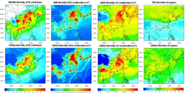
Fig. 4. Comparison between model simulated results and satellite products on 28 March and 13 April 2006, respectively. The evaluated
satellite products include AOD, column NO2 and CO concentration (molecules cm−2)and O3 concentration (ppbv) at around 820 hPa.
AOD was retrieved from the composite Aqua/MODIS C005 using the Deep Blue algorithm at 550 nm and gridded to 0.5×0.5◦resolution.
Column NO2concentration was retrieved from Ozone Monitoring Instrument (OMI) aboard NASA’s EOS Aura satellite. Column CO
concentration was retrieved from the Atmospheric Infrared Sounder (AIRS), and O3concentrations was retrieved from the Tropospheric
Emission Spectrometer (TES).
intensive episodes were chosen, i.e. 27–28 March and 13–14 April.
4.2.2 Remote sensing observations
Besides the model evaluation from ground-based observa-tion, we also evaluated the regional consistence between model results and remote sensing map during the two in-tensive biomass burning episodes as stated above. Figure 4 compares the regional distribution of the observed satellite parameters with the simulated results, including Aerosol
Op-tical Depth (AOD), column NO2concentration, column CO
concentration and O3concentration at around 820 hPa. Gaps
in satellite data were mainly due to possible cloud interfer-ence and limited satellite swath. The satellite observations on 28 March and 13 April were selected to evaluate the model performance here.
was converted by multiplying the aerosol chemical species in the CMAQ model with the aerosol extinction coefficients and then integrated with all altitudes. The detailed method was described in Appendix B. The model generally captured the observed magnitude and distribution of MODIS AOD in Fig. 4. The gaps in satellite AOD were mainly due to cloudy scenes and sun glint over the ocean. Both satellite and CMAQ model showed heavy aerosol loading over the biomass burning region in Southeast Asia and in the down-wind areas, suggesting strong biomass burning activities and long-range transport. On 28 March, two main high AOD re-gions were observed and simulated, one in Southeast Asia, which covered large areas extending eastward to the Western Pacific, and the other in a relatively small area located be-tween 25◦N and 30◦N near the Yangtze River Region. As for the second episode (13 April), although no enough satel-lite data was available in downwind areas, the model still simulated a large scale transport of aerosol. However, the level of the long-range transport during the second episode was not as strong as the first one. On 13 April, the model seemed to predict lower AOD values in the northern part of China than the MODIS observation (Fig. 4). This underes-timation was probably due to the lack of a dust module in CMAQ, as dust events derived from the Gobi desert in North-ern China occurred during this period (Huang et al., 2010; Zhang et al., 2010).
There were two enhancement regions of NO2, one in the
Southeast Asia region and the other in the industrialized east-ern part of mainland China. Although the nitrogen oxides were not the main species emitted from biomass burning, high column concentrations of NO2 were still present over
most of Southeast Asia in both the remote sensing data and model simulation. The areas of high column NO2 were
confined to the source regions in Southeast and East Asia (Fig. 4), suggesting negligible long-range transport of the rel-atively short-lived NO2and different sources of NO2in the
two regions. The high column loading of NO2in the
north-eastern part of China and the Pearl River Delta region was observed by various sensors (van der A et al., 2006) and was mainly due to the large consumption of fossil fuels by power plants, industries, and vehicles. Satellite detected higher sig-nals of O3 and CO over the Southeast Asia region,
espe-cially over Burma, Northern Thailand, Vietnam and South-ern China. Compared to observation, the model simulated stronger signals and overestimated around 20–50 % over the most intense fire regions. In addition, the model predicted a more obvious transport pattern from the source region to over the Western Pacific, which is relatively weak from satel-lite. In other parts of the study domain, the model could rela-tively simulate well. The great uncertainty of biomass burn-ing emission should be the major reason for the difficulty in modeling CO and O3over source fire regions.
Figure 5 shows the monthly mean AOD, NO2, CO and
O3plots from both satellite and modeled results. Generally,
the model could well capture the spatial distribution of most
species on the monthly basis. For AOD, the model slightly overestimated in the northern part of Southeast Asia, e.g. Burma, Laos, while underestimated in the southern part of Southeast Asia, mostly in Thailand. Correspondingly, the similar situation could be found in the monthly CO concen-trations. In Burma, obvious overestimation was simulated. The model performance of NO2was the best among the four
species simulated above. The model performed very well in mainland China and simulated very consistent spatial distri-bution to the hot spots in Northern, Eastern China, and the Pearl River Delta region. There were some overestimations of NO2over some limited regions in Southeast Asia. The
rel-atively good model performance of NO2concentrations was
probably due to that its emission factor from biomass burning was relatively low compared to the anthropogenic sources. The simulation of O3performed relatively well above 30◦N,
however, it overestimated below it, especially in Southeast Asia and Southern China. The overestimation could reach about 10–20 ppbv. We suspected that the local biomass burn-ing emission should be responsible for this.
In summary, the model could relatively well simulate the spatial distribution of typical pollutants emitted from biomass burning. In the next section, we will include with and without the biomass burning emission of Southeast Asia in the model to quantitatively assess the regional influences caused by biomass burning.
4.3 Regional influences from biomass burning
4.3.1 Episodic impact from biomass burning
In order to evaluate the impact of biomass burning on the source and the downstream regions, we performed a numeri-cal scenario case without the biomass burning emissions over Southeast Asia in the model to compare to the base case with all the emission. Thus, the differences between the scenario case and the base case represented the contribution from biomass burning. Figure 6 illustrates the regional impact of biomass burning on the CO, O3, and PM2.5concentrations
during the two episodes (27 March and 13 April) in 2006. The color contours denoted the differences between the base case and the scenario case, i.e. the gases and aerosol concen-trations due to biomass burning. Red contoured lines denoted the percentage of the contribution from biomass burning. And the white arrows denoted the wind vectors in the 15th vertical layer at the altitude of 2.4 km. This layer was chosen mainly because of significant long-range transport above it, which would be discussed in the next section.
Fig. 5.The same as Fig. 4, but for monthly average comparison.
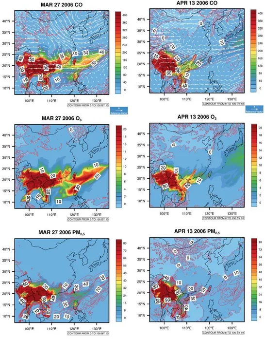
most prominent in the source region of Southeast Asia and over the transport pathways such as the nearby regions of Yunnan and Guangxi provinces in Southern China. In the source regions, biomass burning perturbed concentrations of CO, O3, and PM2.5 by as much as 400 ppbv, 20 ppbv and
80 µg m−3, respectively. The percentages of the above three species attributed to biomass burning were in the ranges of 10 to 60 %, 10 to 20 % and 30 to 70 %, respectively. It seemed that the contribution percentage of O3from biomass burning
was relatively small compared to CO and PM2.5, which was
in agreement with previous results (Zhang et al., 2003). The downwind areas were also strongly influenced by the long-range transport of biomass burning plumes. On 27 March, the impact spread over the southeastern parts of mainland China, including the Pearl River Delta region and Fujian province. The impact from biomass burning on these downwind regions amounted to about 160 to 360 ppbv for CO, 8 to 18 ppbv for O3and 8 to 64 µg m−3for PM2.5. The
biomass burning outflows may also influence Taiwan and even the West Pacific. The transport impact could contribute about 20 to 50 % on CO, 10 to 30 % on O3, and 70 % on
PM2.5, respectively.
Along the major export pathway of the plumes, biomass burning derived CO and O3 were spatially correlated with
each other, probably indicating their common source. The transport pathways of biomass burning derived particles (PM2.5)differed from CO and O3, which diffused quickly
and covered relatively short distances. On 27 March, PM2.5
from biomass burning decreased from 40 to 80 µg m−3over the continent to 8 to 20 µg m−3 over the ocean; thus, over 70 % of the particles were scavenged during the transport. Compared to the gaseous pollutants, particles were more eas-ily subject to scavenge through the wet/dry deposition.
As for the second episode on 13 April (Fig. 6), the im-pacts from biomass burning were not as widespread or in-tense as the first episode. The effects of biomass burning cen-tered over the source region areas of Southeast Asia, South-ern China, and the regions between SouthSouth-ern China and the South China Sea. Beyond the Pearl River Delta region, the impact became less significant, although weak influence of transported plume may still exist over oceanic areas as far as Japan (biomass burning derived CO and O3<100 ppbv and
6 ppbv, respectively with a negligible effect on PM2.5).
4.3.2 Monthly impact from biomass burning
Figure 7 shows the monthly average impact of biomass burn-ing and wind patterns in March and April. In March, biomass burning in Southeast Asia mainly affected southern parts of East Asia. It contributed about 30 to 60 %, 10 to 20 %, and 20 to 70 % of the total CO, O3 and PM2.5 concentrations,
respectively. The long-range transport had a significant im-pact over the Yunnan and Guangxi provinces in China and over the South China Sea around Hainan Island, with 140 to 180 ppbv CO derived from biomass burning. The transported CO extended over broad areas such as the Fujian, Jiangxi, and Hunan provinces in China and the South China Sea. The effect of biomass burning on these regions ranged from 40– 100 ppbv. As for O3, the area influenced was broader than
that of CO, with considerable biomass burning derived O3
concentration of about 8 ppbv in the lower altitudes between 10◦N and 15◦N. There was also a belt over the West Pa-cific with a biomass burning derived O3concentration of 2 to
5 ppbv. The impact of biomass burning on PM2.5was mainly
μ
Fig. 6.Impact of biomass burning in Southeast Asia on 27 March and 13 April 2006. Color contour represents the concentrations for each
species: the top panel shows CO (unit: ppbv) concentration, the middle panel shows O3concentrations (unit: ppbv) and the bottom panel
show PM2.5concentrations (unit: µg m−3). The red contour lines represent percentage contribution from biomass burning. The white arrows denote the wind vectors in the 15th vertical layers at the altitude of 2.4 km.
part of Guangdong and Yunnan provinces, and the South China Sea.
In April, the regional distribution pattern of biomass burn-ing gases and aerosol slightly differed from March as shown in the figure. The impact from biomass burning in April evidently spread over broader regions and even reached the Yangtze River Delta region. For CO, its concentration from biomass burning that reached the Yangtze River Delta region was about 60 ppbv, and accounted for about 10 % of the total
concentration. Additionally, it was simulated that the trans-ported CO concentrations over the South China Sea in April were higher than in March. In the source regions, we didn’t find big differences between the two months. In April, ozone contributed by biomass burning plumes also covered a re-gion broader than that in March. Over most of the Pearl River Delta region, the Guangxi province, and large areas of South China Sea, the O3contribution by biomass
Fig. 7.Similar as Fig. 6 but monthly average impact during March and April in 2006.
of biomass burning on the O3concentrations in parts of the
Fujian, Jiangxi, and Hunan provinces reached about 8 ppbv, about 4 ppbv higher than in March. Another obvious differ-ence was a high O3 concentration belt extending from the
East China Sea to the regions below Japan. The fast dis-persion of O3 was probably related to the prevailing wind
pattern during this period. As for PM2.5, its transport was
also more widespread and influenced major areas of south-ern China; the particulate contribution from biomass burning ranged from 10 to 30 % in downwind areas.
0 2 4 6 8 10 12 14
0 0.1 0.2 0.3
Aerosol extinction (km-1)
He
ig
ht
(
k
m
)
Lidar
CMAQ
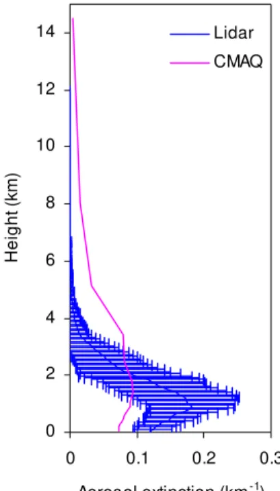
Fig. 8. Vertical distribution of aerosol extinction (km−1) from
both Lidar and CMAQ model at Phimai in Thailand (15.19◦N,
102.56◦E). One standard deviation of Lidar measured aerosol ex-tinction was shown at interval height of every 75 m.
emitted pollutants more northward and eastward, while the South China Sea was less impacted.
4.4 Vertical distribution of biomass plumes
Before we investigate the vertical transport pattern of biomass plumes, it is necessary to evaluate the model per-formance of vertical distribution. Figure 8 shows the com-parison of vertical aerosol extinction between the model and a Micro-Pulse Lidar at Phimai in Thailand (15.19◦N, 102.56◦E). As shown in the figure, the model could gen-erally captured the aerosol vertical distribution. Both lidar and model presented a decreasing trend of aerosol extinc-tion coefficient from the ground to the high altitudes. How-ever, there was underestimation below the PBL (i.e. around 2 km), which could be due to underestimation of local an-thropogenic emission near the ground. Some overestimation was observed at higher altitudes, which could be due to the problem of the allocation method of biomass burning emis-sion. Generally, the vertical distribution of aerosol was rea-sonably well simulated, implying that the modeled vertical results could be further utilized.
Figures 9 and 10 show the simulated altitude-longitude cross-section of CO, O3, and PM2.5from biomass burning
during the two episodes. The color contours and line con-tours denoted as the same meaning as in Fig. 7. The white arrows denoted the wind vectors at different vertical layers.
Two cross-sections at 15◦N and 20◦N were selected and compared, as this region was where the strongest biomass burning occurred. On 27 March at the cross section of 15◦N, we found that there was strong zonal gradient in concen-trations. The blank areas with negligible emissions were over the open oceans. High CO and O3 concentrations in
the boundary layers around 100◦E, 105–110◦E, and 115– 122◦E were noted. At 100◦E and 105–110◦E, the vertical concentration gradient was very small or had an increasing trend from surface to high altitudes, which indicated that the pollutants were emitted from the lands in the source region. Driven by the strong air convection in the tropics, the local emissions lofted to high altitudes and then transported. This is why a plume layer existed at high altitudes of about 2 to 8 km, which extended to around 130◦E via the long range transport.
At around 115–122◦E, an obvious decreasing vertical gra-dient was observed from top to bottom, which suggests con-siderable deposition during the transport of biomass burn-ing plumes. The percentage contributions of the transported plumes from biomass burning were 30 to 50 % for CO, 20 to 40 % for O3and over 70 % for PM2.5from the surface to
al-titude of about 10 km. The cross-section of 20◦N was quite different from that of 15◦N. The zonal gradient in concentra-tions is smaller, as this cross-section covered more land. Pol-lutants started to deposit at around 112◦E, as there was also a decreasing vertical gradient at this longitude. The long-range transport contributed 60 to 70 % to CO, 20 to 50 % to O3, and 80 % to PM2.5from the surface to altitude of about
10 km, respectively.
On 13 April, the transport of the biomass burning plumes was not as strong as on 27 March (Fig. 9), which was also consistent with our previous findings. On the cross-section of 15◦N, the main body of pollutants was located between 98◦E and 110◦E. At the altitudes between 1 km and 5 km, there also existed a plume layer with a short tail that trans-ported to around 120◦E for CO and O3. At the cross-section
of 20◦N, the biomass burning emission intensified. The sub-sidence of pollutants was found at 105–115◦N, which was located at the junction of Vietnam and Guangxi province of China. The air pollutants could be depleted by various path-ways during the subsidence.
As illustrated from the vertical structure of the biomass burning derived species, CO decreased from 400 ppbv at the top to about 160 to 200 ppv, with a depletion percentage of 50 to 60 %. O3decreased from 20 ppbv to 8 to 10 ppbv, also
with a depletion percentage of 50 to 60 %, while PM2.5
μ
Fig. 9. Vertical transport and impact of biomass burning on 27 March 2006 at two cross sections of 15◦N and 20◦N. Color contour
represents the concentrations for each species at each layer. The top panel shows CO (unit: ppbv) concentration, the middle panel shows O3 concentrations (unit: ppbv) and the bottom panel show PM2.5concentrations (unit: µg m−3). The black contour lines represent percentage contribution from biomass burning at each layer. The white arrows denote the wind vectors in each layer.
60 % to 20 %. It seemed that the long-range transport of the biomass plumes exerted greater influence in the free tropo-sphere than in the boundary layer.
5 Conclusions
Fig. 10.Similar as Fig. 7 but for the episode on 13 April 2006.
quality in both local and downwind areas. During the first episode on 27 March, the influence of biomass burning in the source region contributed to CO, O3, and PM2.5
concen-trations as high as 400 ppbv, 20 ppbv, and 80 µg m−3, respec-tively. The reduction percentages of the concentrations on the above three species without biomass burning were in the range of 10 to 60 %, 10 to 20 % and 30 to 70 %, respectively. Also, the impacts due to long-range transport could spread over the southeastern parts of mainland China, including the
Pearl River Delta region and the Fujian province in China. The impact from biomass burning on this region could con-tribute about 160 to 360 ppbv CO, 8 to 18 ppbv O3 and 8
to 64 µg m−3PM2.5, respectively; and the percentage impact
could reach 20 to 50 % on CO, 10 to 30 % on O3, and as high
as 70 % on PM2.5. During the second episode period on 13
The impact of biomass burning derived CO and O3in
South-east Asia and southern China can reached about 100 ppbv and 6 ppbv, respectively, while the impact on PM2.5was not
very significant.
In March, biomass burning in Southeast Asia had signif-icant impact on southern parts of East Asia, especially the Yunnan and Guangxi provinces in China and over the South China Sea. Biomass burning contributed about 30 to 60 %, 10 to 20 %, and 20 to 70 % to the total CO, O3 and PM2.5
concentrations, respectively. In April, due to slightly differ-ent wind patterns, CO effects could reach the Yangtze River Delta with an impact of about 60 ppbv (10 to 20 %). High concentrations of O3extended farther in April. The O3
con-centration reduction ranged from 9 to 11 ppbv in the Pearl River Delta region, the Guangxi province in China, and large areas of the South China Sea. As for PM2.5, its transport was
also more widespread and influenced major areas of southern China, with the particulate contribution from biomass burn-ing ranged from 10 to 30 %.
Two cross-sections at 15◦N and 20◦N were selected to compare the vertical flux of biomass burning. In the source region (Southeast Asia), CO, O3, and PM2.5concentrations
had a strong upward transport from surface to high altitudes. The transport became strong from 2 to 8 km in the free tro-posphere, and the pollutants were quickly transported east-ward due to a strong western wind. The subsidence during the long-range transport contributed 60 to 70 % CO, 20 to 50 % O3, and 80 % PM2.5, respectively, to surface in the
downwind area. Though NASA’s BASE-ASIA conducted this biomass burning measurement, it might be less active in biomass burning in 2006. This modeling study might provide constraints of lower limit. An additional study is underway for an active biomass burning year to obtain an upper limit.
Appendix A
Statistical parameters for evaluating model performance
Some general statistical parameters for model performance evaluation, i.e. MNB (Mean Normalized Bias), MNE (Mean Normalized Gross Error), MFB (Mean Fractional Bias) and MFE (Mean Fractional Gross Error). The calculations are shown in Eqs. (A1)–(A5) below, whereCm andCo are the
simulated model grid value and observational value at time and locationi, respectively. AndN is the total number of samples by time and/or locations. However, as is shown in Eqs. (A1) and (A2), MNB and MNE can become extremely large when the observation data is quite low. For ozone, a cutoff of 40ppb or 60ppb is recommended and this will mini-mize the effect of normalization. MFB and MFE have the ad-vantage of limiting the maximum model/observation bias and error. Benchmarks of MFB and MFE for O3are 15 % and
35 %, respectively. For PM2.5, they are 50 % and 75 %,
re-spectively (USEPA, 2007; Morris, 2005; Morris et al., 2006; Tesche et al., 2006).
MNB= 1
N N X
i=1
Cm−Co
Co
·100 % (A1)
MNE= 1
N N X
i=1
|Cm−Co|
Co
·100 % (A2)
MFB= 1
N N X
i=1
Cm−Co
(Cm+Co)/2
·100 % (A3)
MFE= 1
N N X
i=1
|Cm−Co|
(Cm+Co)/2
·100 % (A4)
The index of agreement (IOA) is calculated by Eq. (A5):
IOA=1−
N P i=1
(Cm−Co)2
N P i=1
(|Cm−Co| + |Co−Co|)2
(A5)
The calculation of Factor 2 is shown in Eq. (A6):
R=N[0.5,2]
Nt
(A6) whereR is the percentage of the ratios between 0.5 and 2; N[1/2,2] is the number of the ratios between 0.5 and 2; and Ntis the total number of comparison points.
Appendix B
Method of calculating AOD from CMAQ model
Aerosol Optical Depth (AOD) used in this study was esti-mated from the concentrations of aerosol chemical species generated from the CMAQ model. AOD was theoretically calculated by integrating the aerosol extinction coefficient (σext(z)) with respect to altitudes (z), i.e.
AOD= ∫σext(z)·dz (B1)
In the CMAQ model, total 19 layers from the surface to 14.4 km were integrated to represent the whole column AOD. We estimated the aerosol extinction coefficient by using an empirical approach known as reconstructed extinction. And this method was proposed by Malm et al. (1994), i.e. σext(Mm−1)=3.0×f (RH)× {[(NH4)2SO4] + [NH4NO3]}
+4.0× [SOAs] +10.0× [BC] +1.0
The numbers in the front of each species were their spe-cific mass extinction efficiency (m2g−1).f(RH) denoted the hygroscopic growth factor, which determined the variability inσext caused by the relative humidity. In the estimation,
only sulfate and nitrate were considered hygroscopic.f(RH) was obtained from a table of corrections with entries at one-percent intervals. The methodology for the corrections was given in Malm et al. (1994).
Acknowledgements. We thank Edward J. Hyer for providing FLAMBE biomass burning emission data. We thank NASA GSFC on funding support (grant no.: NNX09AG75G). Data products from SMART-COMMIT and Deep Blue groups of NASA GSFC are funded by the NASA Radiation Sciences Program, managed by Hal Maring. Hong Kong data was obtained from Hong Kong Environmental Protection Department.
Edited by: F. Yu
References
Air Sciences, Inc.: 2002 Fire Emission Inventory for the WRAP Region – Phase II, Preared for the Western Governors Associa-tion/WRAP by Air Sciences, Inc., Denver, CO, 2005.
Allen, D. J., Kasibhatla, P., Thompson, A. M., Rood, R. B., Dod-dridge, B. G., Pickering, K. E., Hudson, R. D., and Lin, S. J.: Transport-induced interannual variability of carbon monoxide determined using a chemistry and transport model, J. Geophys. Res., 101, 28655–28669, 1996a.
Allen, D. J., Rood, R. B., Thompson, A. M., and Hudson, R. D.: Three-dimensional radon 222 calculations using assimilated me-teorological data and a convective mixing algorithm, J. Geophys. Res., 101, 6871–6881, 1996b.
Andreae, M. O. and Merlet, P.: Emission of trace gases and aerosols from biomass burning, Global Biogeochem. Cy., 15, 955–966, 2001.
Bucsela, E., Celarier, E. A., Wenig, M. O., Gleason, J. F., Veefkind,
J. P., Boersma, K. F., and Brinksma, E. J.: Algorithm for NO2
vertical column retrieval from the Ozone Monitoring Instrument, IEEE Trans. Geosci. Remote Sens., 44, 1245–1258, 2006. Byun, D. W. and Ching J. K. S.: Science algorithm of the EPA
Models-3 Community Multiscale Air Quality(CMAQ) Model-ing System, EPA/600/R-699/030 pp, United States Environmen-tal Protection Agency, Washington, DC, 1999.
Byun, D. and Schere, K. L.: Review of the governing equations, computational algorithms, and other components of the models-3 Community Multiscale Air Quality (CMAQ) modeling system, Appl. Mech. Rev., 59, 51–77, 2006.
Carmichael, G. R., Sakurai, T., Streets, D., Hozumi, Y., Ueda, H., Park, S.U., Fung, C., Han, Z., Kajino, M., Engardt, M., Bennet, C., Hayami, H., Sartelet, K., Holloway, T., Wang, Z., Kannari, A., Fu, J. S., Matsuda, K., Thongboonchoo, N., and Amann, M.: MICS-Asia II: The Model Intercomparison Study for Asia Phase II: Methodology and Overview of Findings, Atmos. Environ., 42, 3468–3490, 2008.
Chand, D., Guyon, P., Artaxo, P., Schmid, O., Frank, G. P., Rizzo, L. V., Mayol-Bracero, O. L., Gatti, L. V., and Andreae, M. O.: Optical and physical properties of aerosols in the bound-ary layer and free troposphere over the Amazon Basin during
the biomass burning season, Atmos. Chem. Phys., 6, 2911–2925, doi:10.5194/acp-6-2911-2006, 2006.
Choi, S. D. and Chang, Y. S.: Carbon monoxide monitoring in Northeast Asia using MOPITT: Effects of biomass burning and regional pollution in April 2000, Atmos. Environ., 40, 686–697, 2006.
Chuang, M. T., Fu, J. S., Jang, C. J., Chan, C. C., Ni, P. C., and Lee, C. T.: Simulation of A Long-range Transport Aerosols from the Asian Continent to Taiwan by a Southward Asian High-pressure System, Sci. Total Environ., 406, 168–179, 2008.
Davidi, A., Koren, I., and Remer, L.: Direct measurements of the effect of biomass burning over the Amazon on the atmo-spheric temperature profile, Atmos. Chem. Phys., 9, 8211–8221, doi:10.5194/acp-9-8211-2009, 2009.
Deng, X. J., Tie, X. X., Zhou, X. J., Wo, D., Zhong, L. J., Tan, H. B., Li, F., Huang, X. Y., Bi, X. Y., and Deng, T.: Effects of Southeast Asia biomass burning on aerosols and ozone concentrations over the Pearl River Delta (PRD) region, Atmos. Environ., 42, 8493– 8501, 2008.
Dickerson, R. R. and Delany, A. C.: Modification of a commer-cial gas filter correlation CO detector for enhanced sensitivity, J. Atmos. Oceanic Technol., 5, 424–431, 1988.
Du, Y.: New Consolidation of Emission and Processing for Air Quality Modeling Assessment in Asia, Master Thesis, Univer-sity of Tennessee, Knoxville, 2008.
Freitas, S. R., Longo, K. M., and Andreae, M. O.: Impact of includ-ing the plume rise of vegetation fires in numerical simulations of associated atmospheric pollutants, Geophys. Res. Lett., 33, L17808, doi:10.1029/2006GL026608, 2006.
Fu, J. S., Jang, C. C., Streets, D. G., Li, Z., Kwok, R., Park, R., and Han, Z.: MICS-Asia II: Evaluating Gaseous Pollutants in East Asia Using An Advanced Modeling System: Models-3/CMAQ System, Atmos. Environ., 42, 3571–3583, 2008.
Fu, J. S., Yeh, F. L., Carey, C. J., Chen, R. J., and Chuang, M. T.: Air Quality Modelling – An Investigation of The Merits of CMAQ In The Analysis of Trans-boundary Air Pollution From Continents to Small Islands, International Journal of Environmental Tech-nology and Management, 10, 22–31, 2009a.
Fu, J. S., Streets, D. G., Jang, C. J., Hao, J., He, K., Wang, L., and Zhang, Q.: Modeling Regional/Urban Ozone and Particulate Matter in Beijing, China, Journal of Air and Waste Management 59, 37-44, 2009b.
Gustafsson, O., Krusa, M., Zencak, Z., Sheesley, R. J., Granat, L., Engstrom, E., Praveen, P. S., Rao, P. S. P., Leck, C., and Rodhe, H.: Brown Clouds over South Asia: Biomass or Fossil Fuel Combustion?, Science, 323, 5913, 495–498, 2009. Guyon, P., Frank, G. P., Welling, M., Chand, D., Artaxo, P., Rizzo,
L., Nishioka, G., Kolle, O., Fritsch, H., Silva Dias, M. A. F, Gatti, L. V., Cordova, A. M., and Andreae, M. O.: Airborne measurements of trace gas and aerosol particle emissions from biomass burning in Amazonia, Atmos. Chem. Phys., 5, 2989– 3002, doi:10.5194/acp-5-2989-2005, 2005.
Experiment and African Monsoon Multidisciplinary Analysis Special Observing Period-0, J. Geophys. Res., 113, D00C17, doi:10.1029/2008JD010077, 2008.
Huang, K., Zhuang, G., Lin, Y., Li, J., Sun, Y., Zhang, W., and Fu, J. S.: Relation between optical and chemical properties of dust aerosol over Beijing, China, J. Geophys. Res., 115, D00K16, doi:10.1029/2009JD013212, 2010.
Hyer, E. J., Allen, D. J., and Kasischke, E. S.: Examining injec-tion properties of boreal forest fires using surface and satellite measurements of CO transport, J. Geophys. Res., 112, D18307, doi:10.1029/2006JD008232, 2007.
IPCC: The Physical Science Basis. Contribution of Working Group I to the Fourth Assessment Report of the Intergovernmental Panel on Climate Change, edited by: Solomon, S., Qin, D., Manning, M., Chen, Z., Marquis, M., Averyt, K. B., Tignor, M., and Miller, H. L., Cambridge University Press, Cambridge, United Kingdom and New York, NY, USA, 2007.
Kim, J., Yoon, S. C., Jefferson, A., and Kim, S. W.: Aerosol hy-groscopic properties during Asian dust, pollution, and biomass burning episodes at Gosan, Korea in April 2001, Atmos. Envi-ron., 40, 1550–1560, 2006.
Kim, S.-W., Chazette, P., Dulac, F., Sanak, J., Johnson, B., and Yoon, S.-C.: Vertical structure of aerosols and water vapor over West Africa during the African monsoon dry season, At-mos. Chem. Phys., 9, 8017–8038, doi:10.5194/acp-9-8017-2009, 2009.
Krotkov, N. A., McClure, B., Dickerson, R. R., Carn, S. A., Li, C., Bhartia, P. K., Yang, K., Krueger, A. J., Li, Z. Q., Levelt, P. F., Chen, H. B., Wang, P. C., and Lu, D. R.: Validation of SO2 re-trievals from the Ozone Monitoring Instrument over NE China, J. Geophys. Res., 113, D16S40, doi:10.1029/2007JD008818, 2008.
Kwok, R. H. F., Fung, J. C. H., Lau, A. K. H., and Fu, J. S.: Numer-ical study on seasonal variations of gaseous pollutants and par-ticulate matters in Hong Kong and Pearl River Delta Region, J. Geophys. Res., 115, D16308, doi:10.1029/2009JD012809, 2010. Leung, F.-Y. T., Logan, J. A., Park, R., Hyer, E. J., Kasis-chke, E. S., Streets, D. G., and Yurganov, L.: Impacts of en-hanced biomass burning in the boreal forests in 1998 on tro-pospheric chemistry and the sensitivity of model results to the injection height of emissions, J. Geophys. Res., 112, D10313, doi:10.1029/2006JD008132, 2007.
Levelt, P. F., Van den Oord, G. H. J., Dobber, M. R., Malkki, A., Visser, H., de Vries, J., Stammes, P., Lundell, J. O. V., and Saari, H.: The Ozone Monitoring Instrument, IEEE Trans. Geosci. Re-mote Sens., 44, 1093–1101, 2006.
Li, C., Krotkov, N. A., Dickerson, R. R., Li, Z. Q., Yang, K., and Chin, M.: Transport and evolution of a pollution plume from northern China: A satellite-based case study, J. Geophys. Res., 115, D00K03, doi:10.1029/2009JD012245, 2010a.
Li, C., Tsay, S. C., Fu, J. S., Dickerson, R., Ji, Q., Bell, S., Gao, Y., Zhang, W., Huang, J., Li, Z., and Chen, H.: Anthropogenic Air Pollution Observed near Dust Source Regions in Northwestern China during Springtime 2008, J. Geophys. Res., 115, D00K22, doi:10.1029/2009JD013659, 2010b.
Li, C., Zhang, Q., Krotkov, N. A., Streets, D. G., He, K. B., Tsay, S. C., and Gleason, J. F.: Recent large reduction in sulfur dioxide emissions from Chinese power plants observed by the Ozone Monitoring Instrument, Geophys. Res. Lett., 37, L08807,
doi:10.1029/2010GL042594, 2010c.
Lin, C.-Y., Hsu, H.-m., Lee, Y. H., Kuo, C. H., Sheng, Y.-F., and Chu, D. A.: A new transport mechanism of biomass burning from Indochina as identified by modeling studies, Atmos. Chem. Phys., 9, 7901–7911, doi:10.5194/acp-9-7901-2009, 2009. Liu, H. Y., Chang, W. L., Oltmans, S. J., Chan, L. Y., and
Har-ris, J. M.: On springtime high ozone events in the lower tropo-sphere from Southeast Asian biomass burning, Atmos. Environ., 33, 2403–2410, 1999.
Malm, W. C., Sisler, J. F., Huffman, D., Eldred, R. A., and Cahill, T. A.: Spatial and Seasonal Trends in Particle Concentration and Optical Extinction in the United-States, J. Geophys. Res.-Atmos., 99, 1347–1370, 1994.
Mari, C. H., Cailley, G., Corre, L., Saunois, M., Atti´e, J.
L., Thouret, V., and Stohl, A.: Tracing biomass burning
plumes from the Southern Hemisphere during the AMMA 2006 wet season experiment, Atmos. Chem. Phys., 8, 3951–3961, doi:10.5194/acp-8-3951-2008, 2008.
Martin, R. V.: Satellite remote sensing of surface air quality, Atmos. Environ., 42, 7823–7843, 2008.
Morris, R. and Koo, B.: Application of Multiple Models to Sim-ulation Fine Particulate in the Southeastern US, National RPO Modeling Meeting, Denver, CO, 2005.
Morris, R. E., Koo, B., Guenther, A., Yarwood, G., McNally, D., Tesche, T. W., Tonnesen, G., Boylan, J., and Brewer, P.: Model sensitivity evaluation for organic carbon using two multi-pollutant air quality models that simulate regional haze in the southeastern United States, Atmos. Environ., 40, 4960–4972, 2006.
Nam, J., Wang, Y., Luo, C., and Chu, D. A.: Trans-Pacific transport of Asian dust and CO: accumulation of biomass burning CO in the subtropics and dipole structure of transport, Atmos. Chem. Phys., 10, 3297–3308, doi:10.5194/acp-10-3297-2010, 2010. Patra, P. K., Ishizawa, M., Maksyutov, S., Nakazawa, T., and
Inoue, G.: Role of biomass burning and climate anomalies for land-atmosphere carbon fluxes based on inverse modeling
of atmospheric CO2, Global Biogeochem. Cy., 19, GB3005,
doi:10.1029/2004GB002258, 2005.
Potter, C., Genovese, V. B., Klooster, S., Bobo, M., and Torregrosa, A.: Biomass burning losses of carbon estimated from ecosystem modeling and satellite data analysis for the Brazilian Amazon region, Atmos. Environ., 35, 1773–1781, 2001.
Reid, J. S., Koppmann, R., Eck, T. F., and Eleuterio, D. P.: A review of biomass burning emissions part II: intensive physical proper-ties of biomass burning particles, Atmos. Chem. Phys., 5, 799– 825, doi:10.5194/acp-5-799-2005, 2005.
Reid, J. S., Hyer, E. J., Prins, E. M., Westphal, D. L., Jianglong, Z., Jun, W., Christopher, S. A., Curtis, C. A., Schmidt, C. C., Eleu-terio, D. P., Richardson, K. A., and Hoffman, J. P.: Global Moni-toring and Forecasting of Biomass-Burning Smoke: Description of and Lessons From the Fire Locating and Modeling of Burn-ing Emissions (FLAMBE) Program, Selected Topics in Applied Earth Observations and Remote Sensing, IEEE Journal of Se-lected Topics in Applied Earth Observations and Remote Sens-ing, 2, 144–162, 2009.
947–973, 2005.
Richter, A., Burrows, J. P., Nuss, H., Granier, C., and Niemeier, U.: Increase in tropospheric nitrogen dioxide over China observed from space, Nature, 437, 7055, 129–132, 2005.
Rissler, J., Vestin, A., Swietlicki, E., Fisch, G., Zhou, J., Artaxo, P., and Andreae, M. O.: Size distribution and hygroscopic prop-erties of aerosol particles from dry-season biomass burning in Amazonia, Atmos. Chem. Phys., 6, 471–491, doi:10.5194/acp-6-471-2006, 2006.
Sherwood, S.: A microphysical connection among biomass burn-ing, cumulus clouds, and stratospheric moisture, Science, 295, 5558, 1272–1275, 2002.
Streets, D. G., Bond, T. C., Lee, T., and Jang, C.: On the future of carbonaceous aerosol emissions, J. Geophys. Res., 109, D24212, doi:10.1029/2004JD004902, 2004.
Streets, D. G., Fu, J. S., Jang, C., Hao, J., He, K., Tang, X., Zhang, Y., Li, Z., Zhang, Q., Wang, L., Wang, B., and Yu, C.: Air quality during the 2008 Beijing Olympic games, Atmos. Environ., 41, 480–492, 2007.
Swap, R. J., Annegarn, H. J., Suttles, J. T., King, M. D.,
Plat-nick, S., Privette, J. L., and Scholes, R. J.: Africa
burn-ing: A thematic analysis of the Southern African Regional Sci-ence Initiative (SAFARI 2000), J. Geophys. Res., 108, 8465, doi:10.1029/2003JD003747, 2003.
Tang, Y. H., Carmichael, G. R., Woo, J. H., Thongboonchoo, N., Kurata, G., Uno, I., Streets, D. G., Blake, D. R., Weber, R. J., Talbot, R. W., Kondo, Y., Singh, H. B., and Wang, T.: Influences of biomass burning during the Transport and Chemical Evolu-tion Over the Pacific (TRACE-P) experiment identified by the regional chemical transport model, J. Geophys. Res., 108, 8824, doi:10.1029/2002JD003110, 2003.
Tan´re, D., Kaufman, Y. J., Herman, M., and Mattoo, S.: Re-mote sensing of aerosol properties over oceans using the MODIS/EOS spectral radiances, J. Geophys. Res., 102, 16971– 16988, doi:10.1029/96JD03437, 1997.
Tesche, T. W., Morris, R., Tonnesen, G., McNally, D., Boylan, J., and Brewer, P.: CMAQ/CAMx annual 2002 performance evalua-tion over the eastern US, Atmos. Environ., 40, 4906–4919, 2006. Thompson, A. M., Witte, J. C., Hudson, R. D., Guo, H., Herman, J. R., and Fujiwara, M.: Tropical Tropospheric Ozone and Biomass Burning, Science, 291, 5511, 2128–2132, 2001.
USEPA: Guidance on the Use of Models and Other Analyses for Demonstrating Attainment of Air Quality Goals for Ozone,
PM2.5and Regional Haze, EPA-454/B-07e002. USEPA, 2007.
van der A, R. J., Peters, D. H. M. U., Eskes, H., Boersma, K. F., Van Roozendael, M., De Smedt, I., and Kelder, H. M.: Detection of the trend and seasonal variation in tropospheric NO2over China, J. Geophys. Res., 111, D12317, doi:10.1029/2005JD006594, 2006.
van der Werf, G. R., Randerson, J. T., Giglio, L., Collatz, G. J., Kasibhatla, P. S., and Arellano Jr., A. F.: Interannual variabil-ity in global biomass burning emissions from 1997 to 2004, At-mos. Chem. Phys., 6, 3423–3441, doi:10.5194/acp-6-3423-2006, 2006.
Wang, S. H., Lin, N. H., Chou, M. D., and Woo, J. H.: Esti-mate of radiative forcing of Asian biomass-burning aerosols dur-ing the period of TRACE-P, J. Geophys. Res., 112, D10222, doi:10.1029/2006JD007564, 2007.
Wang, L., Hao, J., He, K., Wang, S., Li, J., Zhang, Q., Streets, D., Fu, J. S., Jang, C. J., Takekawa, H., and Chatani, S.: Model-ing Study on PM10 Pollution in BeijModel-ing: Regional Contributions and Control Implications, J. Air Waste Manage., 58, 1057–1069, 2008.
Wang, L., Carey, J., Zhang, Y., Wang, K., Zhang, Q., Streets, D., Fu, J., Lei, Y., Schreifels, J., He, K., Hao, J., Lam, Y. F., Lin, J., Meskhidze, N., Voorhees, S., Evarts, D., and Phillips, S.: As-sessment of air quality bene?ts from national air pollution con-trol policies in China. Part I: Background, emission scenarios and evaluation of meteorological predictions, Atmos. Environ., 44, 3442–3448, 2010.
Winkler, H., Formenti, P., Esterhuyse, D. J., Swap, R. J., Helas, G., Annegarn, H. J., and Andreae, M. O.: Evidence for large-scale transport of biomass burning aerosols from sunphotometry at a remote South African site, Atmos. Environ., 42, 5569–5578, 2008.
Xu, J., Zhang, Y., Fu, J. S., and Wang, W.: Process Analysis of Typical Ozone Episode in Summer over Beijing Area, Sci. Total Environ., 399, 147–157, 2008.
Zhang, Y.: Online-coupled meteorology and chemistry models: his-tory, current status, and outlook, Atmos. Chem. Phys., 8, 2895– 2932, doi:10.5194/acp-8-2895-2008, 2008.
Zhang, M. G., Uno, I., Carmichael, G. R., Akimoto, H., Wang, Z. F., Tang, Y. H., Woo, J. H., Streets, D. G., Sachse, G. W., Av-ery, M. A., Weber, R. J., and Talbot, R. W.: Large-scale struc-ture of trace gas and aerosol distributions over the western Pa-cific Ocean during the Transport and Chemical Evolution Over the Pacific (TRACE-P) experiment, J. Geophys. Res., 108, 8820, doi:10.1029/2002JD002946, 2003.
Zhang, Q., Streets, D. G., Carmichael, G. R., He, K. B., Huo, H., Kannari, A., Klimont, Z., Park, I. S., Reddy, S., Fu, J. S., Chen, D., Duan, L., Lei, Y., Wang, L. T., and Yao, Z. L.: Asian emis-sions in 2006 for the NASA INTEX-B mission, Atmos. Chem. Phys., 9, 5131–5153, doi:10.5194/acp-9-5131-2009, 2009. Zhang, W., Zhuang, G., Huang, K., Li, J., Zhang, R., Wang, Q.,