www.atmos-chem-phys.net/10/5515/2010/ doi:10.5194/acp-10-5515-2010
© Author(s) 2010. CC Attribution 3.0 License.
Chemistry
and Physics
Optimal estimation of the surface fluxes of methyl chloride using a
3-D global chemical transport model
X. Xiao1,*, R. G. Prinn1, P. J. Fraser2, P. G. Simmonds3, R. F. Weiss4, S. O’Doherty3, B. R. Miller4, P. K. Salameh4, C. M. Harth4, P. B. Krummel2, L. W. Porter5,†, J. M ¨uhle4, B. R. Greally3, D. Cunnold6,†, R. Wang6, S. A. Montzka7, J. W. Elkins7, G. S. Dutton7, T. M. Thompson7, J. H. Butler7, B. D. Hall7, S. Reimann8, M. K. Vollmer8, F. Stordal9, C. Lunder9, M. Maione10, J. Arduini10, and Y. Yokouchi11
1Department of Earth, Atmospheric, and Planetary Sciences, MIT, Cambridge, MA 02139, USA
2Center for Australian Weather and Climate Research, CSIRO Marine and Atmospheric Research, Aspendale, Victoria, 3195,
Australia
3School of Chemistry, University of Bristol, Bristol, UK
4Scripps Institution of Oceanography, University of California, San Diego, La Jolla, CA 92093, USA
5Center for Australian Weather and Climate Research, Bureau of Meteorology, Melbourne, Victoria, 3000, Australia 6Georgia Institute of Technology, Atlanta, GA, USA
7ESRL, NOAA, Boulder, CO, USA
8Swiss Federal Institute for Materials Science and Technology, Laboratory for Air Pollution/Environmental Technology,
Duebendorf, Switzerland
9Norwegian Institute for Air Research, Kjeller, Norway 10University of Urbino, Urbino, Le Marche, 61029, Italy
11National Institute for Environmental Studies, Tsukuba, Ibaraki, Japan
*now at: Civil & Environmental Engineering, Rice University, Houston, TX 77005, USA †deceased
Received: 28 September 2009 – Published in Atmos. Chem. Phys. Discuss.: 23 December 2009 Revised: 3 June 2010 – Accepted: 4 June 2010 – Published: 22 June 2010
Abstract.Methyl chloride (CH3Cl) is a chlorine-containing
trace gas in the atmosphere contributing significantly to stratospheric ozone depletion. Large uncertainties in esti-mates of its source and sink magnitudes and temporal and spatial variations currently exist. GEIA inventories and other bottom-up emission estimates are used to construct a priori maps of the surface fluxes of CH3Cl. The Model of
Atmo-spheric Transport and Chemistry (MATCH), driven by NCEP interannually varying meteorological data, is then used to simulate CH3Cl mole fractions and quantify the time series
of sensitivities of the mole fractions at each measurement site to the surface fluxes of various regional and global sources and sinks. We then implement the Kalman filter (with the unit pulse response method) to estimate the surface fluxes on regional/global scales with monthly resolution from
Jan-Correspondence to:X. Xiao (xue.xiao@rice.edu)
uary 2000 to December 2004. High frequency observations from the AGAGE, SOGE, NIES, and NOAA/ESRL HATS in situ networks and low frequency observations from the NOAA/ESRL HATS flask network are used to constrain the source and sink magnitudes. The inversion results indicate global total emissions around 4100±470 Gg yr−1with very large emissions of 2200±390 Gg yr−1from tropical plants, which turn out to be the largest single source in the CH3Cl
budget. Relative to their a priori annual estimates, the inver-sion increases global annual fungal and tropical emisinver-sions, and reduces the global oceanic source. The inversion implies greater seasonal and interannual oscillations of the natural sources and sink of CH3Cl compared to the a priori. The
1 Introduction
Methyl chloride (CH3Cl) is the largest, natural source
of stratospheric chlorine, contributing 15–16% of current stratospheric chlorine content (Montzka and Fraser, 2003; Clerbaux and Cunnold, 2006). Methyl chloride is expected to play an increasing role in determining future levels of strato-spheric chlorine as the impact of the anthropogenic Montreal Protocol species declines. The mean mole fraction of CH3Cl
in the remote troposphere is typically 550 ppt (Yokouchi et al., 2000, 2002; Cox et al., 2003; Simmonds et al., 2004). Measurements also show latitudinal variations in CH3Cl
con-centrations, specifically with higher values in the tropics than at the poles (570 vs. 500 ppt, Yokouchi et al., 2000), presum-ably caused by large tropical terrestrial sources. Khalil and Rasmussen (1999) reported a northern tropical seasonal cy-cle with an amplitude of about 10%, while Cox et al. (2003) found a clear but much smaller annual cycle at Cape Grim with an amplitude of 25 ppt (5%), explicable mainly in terms of seasonal changes in the abundance of the hydroxyl (OH) radical, which is the dominant sink of CH3Cl in the
tropo-sphere.
Mole fractions for CH3Cl in firn air from Antarctica
dat-ing back to the early 1900s were only 5–10% lower than the present day (Butler et al., 1999), which is consistent with pre-dominantly natural emissions. Trudinger et al. (2004) also reconstructed CH3Cl levels back to before 1940 from firn
data, and associated its evolution mostly with the biomass burning source. Recent research has focused on identifying and quantifying CH3Cl natural sources and sinks (e.g., Cox
et al., 2004), including newly identified sources from tropical plants (Yokouchi et al., 2002). Keppler et al. (2005) used sta-ble carbon isotope ratios to study and quantify CH3Cl
forma-tion from abiotic methylaforma-tion of chloride, which exists ubiq-uitously in terrestrial ecosystems and results in more CH3Cl
emissions from tropical plants during hot periods (Hamil-ton et al., 2003). The anthropogenic sources (coal combus-tion, incineracombus-tion, and industrial processes) were quantified in the Reactive Chlorine Emissions Inventory (RCEI) (Mc-Culloch et al., 1999) and sum to 160 Gg yr−1(1 Gg=109g), which is only about 5.4% of the total estimated sources. The oceans were once thought to be the dominant source of CH3Cl until the net flux was revised sharply downward
in 1996 by Moore et al. (1996). Current oceanic flux esti-mates account for 20% of the total. Yokouchi et al. (2002) later suggested that CH3Cl emissions from tropical plants
might be the largest known source. They determined that a specific group of ferns and trees in Southeast Asia alone produce 910 Gg yr−1, using the average emission rate from three species of Dipterocarpaceae and the leaf biomass re-ported for mature tropical lowland rainforest. Considering the large variability of CH3Cl emissions among species of a
family and among individual plants of a species, this estimate is expected to have a very large uncertainty. Moreover, only contributions from Dipterocarpaceae in Southeast Asia were
listed in this inventory. Little is known about CH3Cl
emis-sions from Dipterocarpaceae elsewhere in the world, as well as from other CH3Cl-emitting tropical plants. This global
vegetation source certainly warrants additional investigation which is one of the main goals of this paper.
Reaction with the OH radical is the dominant pathway for removal of CH3Cl from the atmosphere, resulting in an
OH-removal “process” lifetime of 1.5 years (a “process” life-time is defined as the total atmospheric content divided by the rate of removal by that process) (Montzka and Fraser, 2003). Other minor loss processes include reaction with chlorine radicals in the marine boundary layer (13-year time), microbially mediated uptake by soils (28-year life-time), and uptake in polar oceans (70-year lifetime). These processes in total result in an atmospheric lifetime of 1.3 years (Montzka and Fraser, 2003), while the latest scientific assessment on ozone depletion stated that the atmospheric lifetime of CH3Cl is 1.0 years based on a revised loss rate
(Clerbaux and Cunnold, 2006). The current best estimate of the magnitude of the identified CH3Cl sources is about
25% less than the best estimate of the magnitude of the better quantified known sinks (Cox et al., 2003). This suggests that there are still missing and/or underestimated CH3Cl sources.
Moreover, due to the complicated natural behavior of the known sources, significant uncertainties exist in their mag-nitudes and in their variations due to seasonal and climatic changes. Using a 3-D global model of atmospheric CH3Cl,
Lee-Taylor et al. (2001) were able to reproduce the obser-vations of Khalil and Rasmussen (1999) by using a mas-sive tropical terrestrial source of∼2380 Gg yr−1and
reduc-ing previous estimates of emissions from Southeast Asia. Yoshida et al. (2006) used a Bayesian least squares inverse method in a 3-D model to constrain hemispheric and seasonal biogenic and biomass burning sources with 3-month resolu-tion. Although the available measurements covered several years, an “average year” was generated for both the mea-surements and the derived sources. The estimated biogenic, biomass-burning, and oceanic sources were 2500 (close to the Lee-Taylor et al. (2001) estimate), 545, and 761 (dou-ble the bottom-up estimate) Gg yr−1, respectively. However, actual month-to-month and interannual variability in these sources related to climatic changes was not resolved by this approach.
To assess the interannual variability as well as seasonal changes in the surface fluxes of CH3Cl, we use the inverse
modeling approach to optimally deduce the magnitudes of the surface fluxes of CH3Cl from chosen regions and
pro-cesses between 2000 and 2004 at monthly time resolution. In particular, we adapt the Kalman filter for estimating time-varying sources and apply it in a 3-D chemical transport model by using the CH3Cl surface observations from
2 Observations
The accuracy of the inverse modeling is highly dependent on the availability, accuracy and precision of the measurements. We use both high frequency in situ and low frequency flask observations of the mole fractions of CH3Cl. These two
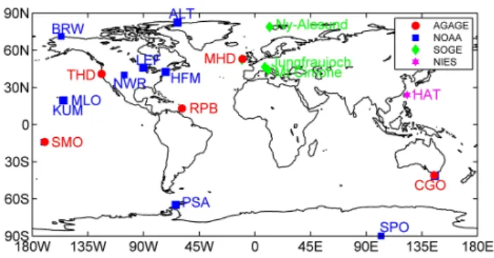
sam-pling strategies represent two complementary approaches to global sampling: high sampling frequency (in situ) and high spatial coverage (flasks). High frequency in situ CH3Cl
mea-surements are available from: the Advanced Global Atmo-spheric Gases Experiment (AGAGE) (Prinn et al., 2000); the System for Observation of Halogenated Greenhouse Gases in Europe (SOGE) and the National Institute for En-vironmental Studies (NIES) in Japan, which are both affil-iated with AGAGE; and the Halocarbons and other Atmo-spheric Trace Species (HATS) In Situ Monitoring Program of NOAA/ESRL (http://www.esrl.noaa.gov/gmd/hats/insitu/ cats/). Low frequency observations are available from the HATS Flask Sampling Program at NOAA/ESRL (Montzka et al., 1999, 2000) and from NIES. Figure 1 shows the loca-tions of the observing sites used in this study, and additional information is listed in Table 1. We used observations from January 2000 to November 2005 from these networks (where available) in order to estimate the monthly surface fluxes during 2000–2004. In this time frame, AGAGE data were from two instruments, the ADS GC-MS (gas chromatograph-mass spectrometer with an adsorption-desorption system) for 2000–2004 and the Medusa GC-MS for 2005; the two instru-ments were intercompared (and agreed well), and used the same calibration scale. We used high frequency data with obvious pollution events removed but the difference between removing and not removing these events is important only at MHD and CGO. At the remote sites the difference is negligi-ble (e.g., monthly means with pollution are on average only 0.19% larger than without pollution at JUN; this is much less than the overall observational errors discussed later).
The networks listed in Table 1 are using different cali-bration scales. The AGAGE and SOGE networks use the AGAGE Scripps Institution of Oceanography 2005 (SIO-05) CH3Cl scale. Regular comparisons of data between
AGAGE/SOGE and the other networks provide estimates of the ratios of the scales used by the other laboratories to the SIO-05 scale (Krummel et al., 2009) as shown in Table 1. While an objective assessment of the errors in these inter-network ratios is not available, we have tested the sensitiv-ity of our inversions to errors in these ratios by repeating the inversions assuming that the percentage differences in mole fractions between AGAGE and each of the other net-works are a significant factor of 1.5 (i.e., 50%) larger than the Krummel et al. (2009) values (see Table 1 for adjusted ratios and Sect. 5.3 for discussion of the results of the inversions us-ing these adjusted ratios). We note that the actual differences between the networks are only 0.6 to 2% for CH3Cl.
Fig. 1. Location of CH3Cl observing sites from different surface networks.
Our inverse methods use monthly mean mixing ratios (χ )
Table 1.Location of the CH3Cl measuring sites and their assumed calibration factors (CF) relative to the SIO-05 CH3Cl scale used by the AGAGE network. Data at each site were divided by the listed calibration factor in order to combine them under a common scale. Calibration factors in parentheses are used in a sensitivity exercise and are calculated by multiplying the interlaboratory differences (CF-1) by 1.5 (i.e., increasing the differences by 50%).
Number ID Location Latitude Longitude Altitude Network Calibration factor (CF) High Frequency Observations
1 MHD Mace Head, Ireland 53.3◦N 9.9◦W 25 AGAGE/SOGE 1 2 THD Trinidad Head, California 41.0◦N 124.0◦W 140 AGAGE 1 3 RPB Ragged Point, Barbados 13.0◦N 59.0◦W 42 AGAGE 1 4 CGO Cape Grim, Tasmania 41.0◦S 145.0◦E 94 AGAGE 1 5 JUN Jungfraujoch, Switzerland 46.5◦N 8.0◦E 3580 SOGE 1 6 MTE Monte Cimone, Italy 44.2◦N 10.7◦E 2165 SOGE 1 7 ZEP Zeppelin Station, Norway 78.9◦N 11.9◦E 474 SOGE 1
8 HAT Hateruma, Japan 24.1◦N 123.8◦E 47 NIES 1.0100 (1.0150) 9 BRW Pt. Barrow, Alaska 71.3◦N 156.6◦W 8 NOAA 1.0212 (1.0318) 10 MLO Mauna Loa, Hawaii 19.5◦N 155.6◦W 3397 NOAA 1.0212 (1.0318) 11 NWR Niwot Ridge, Colorado 40.0◦N 105.5◦W 3018 NOAA 1.0212 (1.0318) 12 SMO Cape Matatula, American Samoa 14.3◦S 170.6◦W 77 NOAA 1.0212 (1.0318) 13 SPO South Pole, Antarctica 89.9◦S 24.8◦W 2810 NOAA 1.0212 (1.0318)
Low Frequency Observations
14 MHD Mace Head, Ireland 53.3◦N 9.9◦W 25 NOAA 1.0102 (1.0153) 15 CGO Cape Grim, Tasmania 41.0◦S 145.0◦E 94 NOAA/NIES 1.0102 (1.0153) 16 THD Trinidad Head, California 41.0◦N 124.0◦W 140 NOAA 1.0102 (1.0153) 17 HAT Hateruma, Japan 24.1◦N 123.8◦E 27 NIES 1.0064 (1.0096) 18 ALT Alert, Northwest Territories, Canada 82.5◦N 62.5◦W 210 NOAA 1.0102 (1.0153) 19 BRW Pt. Barrow, Alaska 71.3◦N 156.6◦W 11 NOAA 1.0102 (1.0153) 20 LEF WLEF tower, Wisconsin 46.0◦N 90.3◦W 470 NOAA 1.0102 (1.0153) 21 HFM Harvard Forest, MA 42.5◦N 72.2◦W 340 NOAA 1.0102 (1.0153) 22 NWR Niwot Ridge, Colorado 40.1◦N 105.6◦W 3472 NOAA 1.0102 (1.0153) 23 MLO Mauna Loa, Hawaii 19.5◦N 155.6◦W 3397 NOAA 1.0102 (1.0153) 24 KUM Cape Kumukahi, Hawaii 19.5◦N 154.8◦W 3 NOAA 1.0102 (1.0153) 25 SMO Cape Matatula, American Samoa 14.2◦S 170.6◦W 77 NOAA 1.0102 (1.0153) 26 PSA Palmer Station, Antarctica 64.9◦S 64.0◦W 10 NOAA 1.0102 (1.0153) 27 SPO South Pole, Antarctica 89.98◦S 102.0◦E 2841 NOAA 1.0102 (1.0153)
We use the 3-D model output to estimate the sampling fre-quency and mismatch errors following the approach of Chen and Prinn (2006).
There is generally a lower uncertainty associated with the high frequency measurements (e.g., 1.5% on average) due to their capability to better capture sub-monthly temporal variations and thus better define monthly means. Although the monthly means from flask measurements therefore have larger assigned errors (e.g., 2.4% on average) than those from the high frequency measurements (i.e., they have larger error covariance matrices,R; see Appendix A), the greater prox-imity of some of the flask sites to some of the emitting re-gions can make them more sensitive to those rere-gions (i.e., they can have larger sensitivity matrices, H; see Sect. 4) which can help offset the effects of larger Rin the calcu-lation of the Kalman gain matrix,K, that determines the ef-fectiveness of each measurement in improving the emission estimates (see Appendix A).
3 The MATCH model
a hybrid coordinate, which consists of a terrain-following sigma coordinate combined with (optional) constant pres-sure level values. The NCEP data are on 28 sigma levels. The model time step is 40 min for the T42 resolution. The archived data are linearly interpolated between the neighbor-ing time intervals to obtain the values for each time step.
Although MATCH can be extended to simulate the com-plicated photochemistry in the atmosphere (e.g., Lawrence et al., 1999; von Kuhlmann et al., 2003; Lucas and Prinn, 2005), only simple chemistry using offline OH concentra-tions needs to be incorporated into the basic MATCH model for the simulation of CH3Cl because it is not a major sink
for OH or source of HOx. The predominant removal process
in the troposphere for CH3Cl is oxidation by the OH radical,
which is the primary oxidizing chemical in the atmosphere. The relevant reaction is (Sander et al., 2006):
CH3Cl+OH→CH2Cl+H2O (R1)
The temperature-dependent rate constant for reaction with the OH radical is given in the Arrhenius form:
k(T )=Aexp[(−E/R)(1/T )] (R2)
where A is the pre-exponential factor
(=2.4×10⁻¹²cm3molecule−1s−1), R is the univer-sal gas constant, E is the activation energy (J mol−1)
(E/R=1250 K) (Sander et al., 2006), and T(K) is the temperature. In the model simulation,k(T )is updated each time step based on the ambient conditions (temperature, pressure, etc.) in the grid cells.
The offline OH fields chosen are from the output gen-erated using the version of MATCH-MPIC described in Lawrence et al. (1999), J¨ockel (2000), and von Kuhlmann et al. (2003). This MATCH version incorporates a full photo-chemical component, representing the major known sources (e.g., industry, biomass burning), transformations (chemical reactions and photolysis), and sinks (e.g., wet and dry depo-sition) for studies of ozone and hydrocarbons in the tropo-sphere. Chen and Prinn (2005, 2006) used the monthly mean MATCH-MPIC 3-D OH fields at T63 resolution adjusted to fit global AGAGE methyl chloroform (CH3CCl3)
observa-tions (we reduced these T63 fields to T42 for this work). Fi-nally, a diurnal cycle linked to the solar zenith angle is further applied to the daily average OH concentrations interpolated by MATCH from the monthly mean OH concentrations. This ensures zero nighttime values while maintaining the daily average OH concentrations (Chen and Prinn, 2005, 2006). Since the annual and global average OH did not change much (within 3%) over the period of 2000–2004 (Fig. 2, Prinn et al., 2005), we used annually repeating OH fields. This allows us to assess the effect of the interannually varying transport (captured in the NCEP data) on the concentrations of CH3Cl.
In the stratosphere, CH3Cl is oxidized by the hydroxyl
rad-ical and also photodissociates. However, the stratospheric sink is small for CH3Cl (7.6% of the total atmospheric loss,
Cox et al., 2003), and most of the stratospheric loss arises from OH attack (Seinfeld and Pandis, 1998), which is ac-counted for by the above 3-D OH fields in MATCH. Pho-todissociation of CH3Cl in the stratospheric is neglected in
the model due to its very small role relative to OH as a global sink of CH3Cl.
4 Methodology for inverse modeling
The inversion methodology used follows the approach of Chen and Prinn (2006) and the detailed methodology is de-scribed in Appendix A. The method is based on the Kalman filter (Prinn, 2000), which is adapted to estimate time-varying fluxes at monthly resolution for transient sources and invariant aseasonal fluxes for more steady sources. For this purpose, it is adequate to use monthly mean observations to constrain the monthly surface fluxes. What we actually es-timate are the magnitudes of the regional or global fluxes by location and/or process, assuming we know their spa-tial distributions within each region (referred to here as the reference or a priori maps). Specifically, the state vectorx
in the Kalman filter contains variables representing the re-gional or global magnitudes of the surface fluxes of CH3Cl
for the time period of 2000–2004 with month-to-month vari-ations allowed for seasonal processes. In the adaptation of the Kalman filter, the full state vector including the elements for the surface fluxes of the total 60 months is truncated when using the observations step by step (see Appendix A).
We use the MATCH model to compute the sensitivities (the matrixH)of the mole fractions at different sites to the state vector elements by finite differences. A straightforward approach for computingHfor ann-dimensional state vector
xis to do a single model run withn+1 chemically identical (but separately labeled) chemical species. One of the chem-ical species uses a reference (e.g., a priori best estimate) of
x, while the othernspecies use values ofxwith one element slightly perturbed from its reference value.
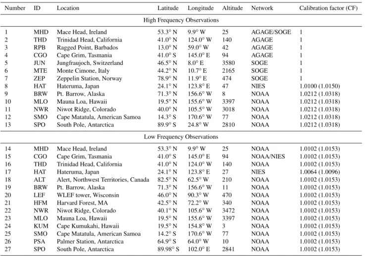
Fig. 2.MATCH-modeled sensitivities of CH3Cl(a)high frequency and(b)monthly mean mole fractions at each AGAGE site to a January 2000 emission pulse from African tropical plants. Eventually the mole fractions reach similar values for each site consistent with a CH3Cl emission pulse into a well-mixed atmosphere. In addition to dispersion, the sensitivities are affected by a slow CH3Cl decrease due to reaction with the OH radical.
decays due to atmospheric dispersion and chemical loss. We call this the “unit pulse method”. For the period of 2000– 2004 we have performed 5 years×12 months=60 monthly pulse runs, each being a separate multi-tracer run starting at a different month. The global mixing (dispersion) time in the model is about one year (Chen and Prinn, 2006). Therefore we run each of the 60 monthly pulses for 12 months instead for the full 2000–2004 period with the pulse affecting only the global average after 12 months.
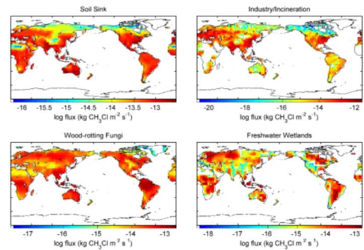
Figure 2 shows examples of calculated sensitivities for in-dividual sites to an inin-dividual monthly pulse as functions of time, specifically a January 2000 uniform emission pulse of 10 Gg yr−1 from the tropical plants in Africa. Results are
shown at: (a) the model time resolution and (b) the monthly time resolution of the deduced fluxes. The sensitivities are largest in the first 3–4 months and then decrease because of dispersion due to atmospheric mixing. Responses at differ-ent sites show differdiffer-ent behaviors because of their differdiffer-ent location relative to the source region and due to the global wind patterns. Ragged Point, Barbados and Cape Matatula, American Samoa are located in the tropical east wind region and are downwind of Africa, and therefore respond rapidly to the plant emission pulse with sharp peaks. Ragged Point is closer to Africa than Cape Matatula, and shows the more rapid response. The other three sites are either further away from the source region and/or not in the same wind regime as the source region. Therefore their responses are less sharp and relatively slow. All the responses include continuous de-creases due to reaction of CH3Cl with the OH radical. Note
that the responses at different sites tend to converge to a sin-gle value after one year which is consistent with an emission pulse into a well-mixed atmosphere. These monthly seasonal sensitivities, along with the monthly aseasonal sensitivities, are used to construct the time dependent sensitivity matrixH
used in the inversions.
5 Inversion for methyl chloride
In this section we present inversion results for CH3Cl surface
fluxes using the methodology described in Sect. 4. The op-timized surface fluxes include seasonal, annual, and interan-nual values for specific emitting and depleting processes and regions. The inversion results are presented and discussed in sequence, with a particular emphasis on possible emission and depletion anomalies associated with the 2002/2003 glob-ally wide-spread heat and drought which was partly caused by the minor 2002/2003 El Ni˜no event. We also test the sen-sitivity of the inversion results to different combinations of observations.
5.1 Definition of the state vector and its a priori flux maps
In the inverse modeling methodology, a priori flux distribu-tions are needed as the initial guesses for the unknown sur-face fluxes. It is important to know the spatial distributions of the reference regional or process-based fluxes as accu-rately as possible, but not their magnitudes or time depen-dence since these will be estimated in the inversion.
Page 1/ 1
Fig. 3.Annual average distributions of reference CH3Cl emissions. Emission magnitudes and patterns vary by month. Tropical plants (America, Asia, and Africa) and biomass burning (East and West) have been further subdivided for the inversion. Note that the maps are on a log scale except for the oceans which have a linear scale.
reference year 1990. Lee-Taylor et al. (2001) modified and extended these estimates in their 3-D modeling of CH3Cl by
parameterizing month by month seasonal variations. These emissions represent our best initial guess of CH3Cl fluxes
before optimization of individual regions or processes. As suggested by Yokouchi et al. (2002), CH3Cl emissions
from tropical plants might be the largest known source, but they are not included in this GEIA inventory. We assumed in this study that tropical plants have a significant role in CH3Cl
production and incorporated this process into the inversion to estimate its magnitude and seasonality on regional scales. For our reference emissions, we attribute the imbalance of the global CH3Cl budget between known sources and sinks
(Cox et al., 2003) to this tropical plant process and spatially distribute the resulting global emission estimate proportion-ally to published net primary productivity (NPP) estimates of tropical plant ecosystems in each MATCH grid square (McGuire et al., 2001). The measurements of Yokouchi et al. (2000) show close correlations between local enhance-ments of CH3Cl and a biogenic compoundα-pinene,
emit-ted by tropical plants. Foliar emissions ofα-pinene have been argued to be proportional to foliar density, tempera-ture, and available light (Guenther et al., 1995). Therefore it is reasonable to assume that CH3Cl fluxes are also
pro-portional to the foliar density of the emitting plants. Guen-ther et al. (1995) furGuen-ther argue that foliar density is propor-tional to the NPP of the relevant species. The monthly trop-ical plant NPP database (0.5◦×0.5◦ latitude, longitude) es-timated by McGuire et al. (2001) represents the net produc-tion of organic matter in tropical ecosystems and accounts for the influences of atmospheric CO2, and seasonal and climatic
changes in temperature, precipitation, and available light. These flux maps have been interpolated to the MATCH T42 grid system (2.8◦×2.8◦)while conserving their global
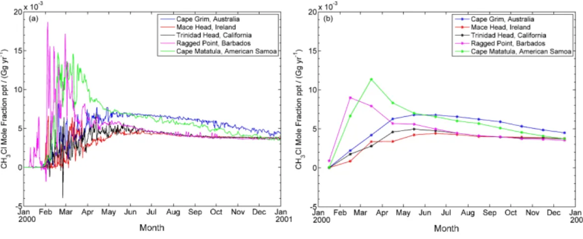
Fig. 4. Annual average distributions of additional CH3Cl monthly varying emissions and the soil sink. Note that the small industrial, incineration and wetland sources are assumed to be equal to their reference values and are not estimated. Seasonal variability of the small fungal emissions is not considered in the inversion.
magnitudes by using the SCRIP (Spherical Coordinate Remapping and Interpolation Package) software. Figures 3 and 4 show the annually averaged reference spatial distri-butions of the surface fluxes from tropical plants, oceans, biomass burning, anthropogenic activities, and other pro-cesses. Tropical emissions are divided into three regions, America, Asia, and Africa, for the inversions, denoted as Trop AM, Trop AS, and Trop AF, respectively. Emis-sions from biomass burning are further divided into Western (North and South America) and Eastern (Africa (including West Africa), Europe (including Spain), Asia, and Australia) regions, denoted as BB West and BB East, respectively. Oceans are a source at lower latitudes and a sink at higher latitudes for CH3Cl and correction factors for its reference
map are only estimated globally. We also estimate correction factors for the maps of global emissions from salt marshes and the global uptake rates by soils (soil sink). Emissions from freshwater wetlands are very small and are kept at their reference values with assumed seasonal changes that are not estimated here. Seasonal variations of the relatively small fungal emissions are not considered here (as in Lee-Taylor et al., 2001) and its global emissions are solved only as an aseasonal flux. The small annual industry/incineration flux is not estimated here because of its spatial correlation with the fungal emissions. The corresponding state vector at time
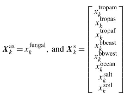
kcan be expressed as:
xk=
Xask Xsk Xsk−1
...
Xsk−T
WhereT=11 months (see Appendix A),
Xask =xkfungal,andXsk=
xktropam xktropas xktropaf xkbbeast xkbbwest xoceank
xksalt xsoilk
(2)
We use data and calculate estimates for the period from 2000 to 2004 (total of 60 months). The global magnitudes of the reference emissions and their mode of incorporation in the state vector are listed in Table 2. The a priori errors for the state vector elements are ±30% to ±50% of their refer-ence values. If both high frequency in situ data and low fre-quency flask data are available for the same site, the high frequency measurements were chosen as they capture intra-monthly temporal variations much better.
5.2 State vector evolution
The equations used in the Kalman filter inversions are given in Appendix A (Prinn, 2000). There are hundreds of monthly flux elements in the state vector, but to illustrate the inver-sion process we focus here on a subvector representing a sin-gle month of fluxes (specifically September 2002). Figure 5 shows the evolution of this subvector, or equivalently how the estimates for the fluxes in a given single month change with each new month of data. As mentioned before, only 12 months of subsequent observations are used to constrain the fluxes of a given single month. The adjustments to the ref-erence value (unity) are shown, so the initial value for each seasonal process is therefore zero with a generous a priori (blue) error bar of either±30% or ±50% depending on our subjective estimate of the quality of the a priori data and the expected year-to-year variability. With each new month of observations, the adjustments change and the error decreases. The amount of the error decrease depends on the errors in the data (Rmatrix, see Appendix A) and on the sensitivities of each observing station to the emissions (Hmatrix, see Ap-pendix A) for each emission region or process. Note that the changes and the error reductions for a given process are greatest in the first few months, because the strongest sensi-tivities of the observations to the emission pulse occur in that time frame. In the final few months, the estimated flux val-ues and uncertainties stabilize even with the addition of new data. The optimized inversion results for September 2002 fluxes are the final values in Fig. 5. These final (a posteriori) values represent the adjustments to the reference (a priori) fluxes that minimize the estimation error variances. As noted earlier, because only 12 months of data have been used, these final values are phased out of the inversion and stored when a new subvector (in this case representing September 2003
Fig. 5.The recursive estimation of CH3Cl surface fluxes for a single month (September 2002) obtained with the use of monthly observa-tions from September 2002 to August 2003 (horizontal axis). The vertical axis corresponds to the dimensionless adjustment from the reference value (unity). The blue line shows the a priori error bar (either±0.3 or±0.5) for the September 2002 surface flux. The fi-nal optimized results are taken as the values at the last step at which time the inversion has stabilized.
fluxes) enters the inversion process. The optimized estimates are then tested using a forward run of MATCH which is com-pared to the observations. These tests will be presented after the inversion results.
5.3 Inversion results
Here we present the results with all of the available obser-vations used in the Kalman filter (i.e., all AGAGE, NOAA, NIES and SOGE in situ data plus all NOAA and NIES flask data at sites where there are no in situ measurements). We have also tested the sensitivities of the inversion results to the chosen data by using several different subsets of the ob-servations from the various networks (see Sect. 5.3.2).
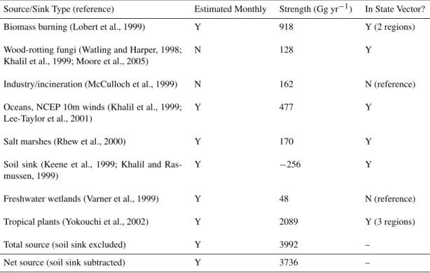
Table 2.Reference annual average strengths of the sources and sinks of CH3Cl and their incorporation in the inversion. Y=YES and N=NO.
Source/Sink Type (reference) Estimated Monthly Strength (Gg yr−1) In State Vector?
Biomass burning (Lobert et al., 1999) Y 918 Y (2 regions)
Wood-rotting fungi (Watling and Harper, 1998; Khalil et al., 1999; Moore et al., 2005)
N 128 Y
Industry/incineration (McCulloch et al., 1999) N 162 N (reference)
Oceans, NCEP 10m winds (Khalil et al., 1999; Lee-Taylor et al., 2001)
Y 477 Y
Salt marshes (Rhew et al., 2000) Y 170 Y
Soil sink (Keene et al., 1999; Khalil and Ras-mussen, 1999)
Y −256 Y
Freshwater wetlands (Varner et al., 1999) Y 48 N (reference)
Tropical plants (Yokouchi et al., 2002) Y 2089 Y (3 regions)
Total source (soil sink excluded) Y 3992 –
Net source (soil sink subtracted) Y 3736 –
oscillations than seen in the reference for almost all of the seasonal processes.
The optimized fluxes also show significant interannual variability, of which the flux anomalies for the period of 2002/2003 for several processes are noteworthy. There were unusual 2002/2003 decreases in CH3Cl emissions from
American tropical ecosystems, unusually high emissions from the eastern biomass burning source in the late spring of 2002/2003, unusually large emissions from the western biomass burning source in late 2002, an anomalous emission rise from global salt marshes in the summer of 2002 through early 2003, and an unusual reduction in the global soil uptake in the northern summer of 2003.
These anomalies are likely attributable to the significant 2002/2003 globally wide-spread heat waves and droughts which were partly associated with the 2002/2003 El Ni˜no that lasted from September 2002 to August 2003. Recent studies show a consistent link between El Ni˜no and drought in the tropics (Lyon, 2004) and mid-latitudes (Zeng et al., 2005). While the El Ni˜no during this time was moderate compared to the extreme 1997/1998 El Ni˜no, the period of 2002/2003 appears unusual because global land precipitation was very low, leading to very dry and hot conditions (Knorr et al., 2007).
Ciais et al. (2005) deduced that there was a reduction in net plant primary productivity apparently caused by the heat and drought in 2003. This reduction in primary productivity is the probable cause of the reductions in tropical plant
emis-sions because of the correlation of primary productivity and foliar emission as noted earlier (Guenther et al., 1995).
The extremely dry and hot season might also lead to in-creased insect damage to vegetation and inin-creased suscepti-bility of the boreal biome to fire (Kobak et al., 1996; Ayres and Lombardero, 2000). Using measurements of burned for-est area in Central Siberia (approx. 79–119◦E, 51–78◦N), Balzter et al. (2005) showed that 2002 and 2003 were the two years with the largest fire extent in Central Siberia since 1996. This is the region within our Biomass Burning (BB) East map. These enhanced fire events are expected to in-crease CH3Cl emissions. This is supported by the study
of Simmonds et al. (2005), which shows that Siberian fires caused a growth rate anomaly in Mace Head baseline CH3Cl
values in 2002–2003.
Page 1/ 1
Fig. 6.Inversion results for the eight seasonally varying processes for emissions of CH3Cl. Blue lines show the reference magnitudes, which are annually repeating. Red lines show the optimized esti-mates, which show interannual variability. The total value is the sum of the emissions from the eight seasonal processes, the as-sumed time invariant aseasonal fungal emissions, and the reference industrial and wetland emissions.
Methyl chloride is degraded in soils by microbial activ-ity. Lee-Taylor et al. (2001) parameterized soil uptake of CH3Cl by assuming proportionality to a methyl bromide
(CH3Br) soil sink extrapolation (Lee-Taylor et al., 1998).
The latter approach used CH3Br observations of Shorter et
al. (1995) and assumed a microbial activity/soil temperature relationship (Cleveland et al., 1993; Holland et al., 1995) with stronger microbial activity at higher temperatures. This is why the reference global soil uptake rate is greatest in the summer of the Northern Hemisphere. However, the in-version indicates an unexpected decrease of the soil sink in the summer of 2003. The microbial activity/soil temperature relationship neglects the influence of soil moisture on mi-crobial activity and uptake efficiency. Laboratory and field experiments by Shorter et al. (1995) did show a general rela-tionship of decreasing CH3Br uptake activity with decreasing
moisture and organic matter content. Therefore the anoma-lously low global soil uptake might have been caused by the extremely widespread drought conditions in 2003.
If future climate in the Northern Hemisphere evolves to-ward increasingly dry and hot summers caused by a substan-tial increase in variability of temperature and precipitation in response to greenhouse forcing (e.g., Sch¨ar et al., 2004), this may lead to increased probability of decreased NPP (and hence decreased tropical CH3Cl emissions), increased
sions from biomass burning, increased salt marsh plant emis-sions, and decreased soil organic matter and microbial activ-ity (and hence decreased CH3Cl consumption by soils).
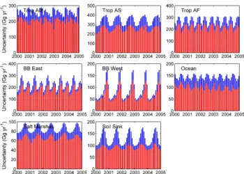
Figure 7 shows the corresponding uncertainties of the op-timized estimates by superimposing the opop-timized (a posteri-ori) uncertainties (red bars) on top of the reference (a priposteri-ori) uncertainties (blue bars). Note that the inversion always
re-Fig. 7.The corresponding uncertainties (1σerror bars) of the inver-sion results in Fig. 6, with the optimized error bars (red) superim-posed upon the reference error bars (blue).
duces the initial uncertainty by amounts depending on the value of the observations in constraining each emission pro-cess or region. Uncertainties for Trop AS plants, Oceans, and the Soil Sink decrease the most, those for Trop AF plants, BB West, and Salt Marshes have smaller reductions, while those for Trop AM plants and BB East have the least reductions, relative to their corresponding initial uncertainties.
As noted in Sect. 2, we also carried out inversions using adjustments to the best-estimate calibration ratios between the networks (see Table 1), in order to ascertain the sensitiv-ity of our inversions to these ratios. The sensitivsensitiv-ity is very small with the average root-mean-square percentage differ-ence between the emission estimates with and without the adjustments being only 2%. This is due both to the small dif-ferences between the network calibrations, and to the domi-nant contribution of the mismatch or representation error on the overall measurement error used in the inversions.
Fig. 8.Five-year averaged results for the 8 seasonally varying emis-sion processes of CH3Cl. Blue lines show the reference magnitudes. Red lines show the optimized estimates.
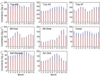
5.3.1 Average seasonal results
To obtain a single representative seasonal cycle for each sea-sonally varying process, we calculated the arithmetic average of each month during the five year period. The corresponding associated uncertainties are
¯
σt= v u u u t
N P
1
σt,n2
N (3)
wheretrepresents a particular month (e.g., January) andn=
1 toN=5, for the five years of the inversion.
Figure 8 shows the averaged seasonal cycle results (red lines) compared to the reference ones (blue lines), and Fig. 9 shows their corresponding uncertainties. For the tropical plant emissions, the seasonal variations differ somewhat from the reference for the three regions, with the most sig-nificant differences occurring for the tropical American re-gion which exhibits two emission peaks. One is in January (its reference value shows a peak in December) and the other one is in August. As noted earlier, the variability in tropical emissions is the net of the combined influences of the vari-ables atmospheric temperature, precipitation, and available light, and therefore does not generally reflect the annual cy-cle of one of these variables alone. While emissions from tropical plants in Africa have a maximum in December, they have a minimum in July. This is probably because at this time Africa is very dry and plant growth activity (NPP) is inhibited.
Deduced biomass burning emissions retain approximately the temporal variations present in their a priori (reference) values. To study the seasonal behavior of the biomass burn-ing source, we examine in Fig. 10 the partitionburn-ing of the de-duced seasonal cycles of the Eastern and Western sources
Fig. 9.The corresponding uncertainties (1σerror bars) of the inver-sion results in Fig. 8, with the optimized error bars (red) superim-posed upon the reference error bars (blue).
Fig. 10. Partitioning of the deduced average seasonal cycles of the Eastern and Western biomass burning sources into the Northern and Southern Hemispheres. Note the dominance of the Eastern North-ern Hemispheric emissions of CH3Cl. Also note the emission peaks of the Northern and Southern Hemispheres occur in the respective spring seasons consistent with dry conditions leading to increase biomass burning activity.
Table 3.Reference and optimally estimated five-year averaged surface fluxes and their errors for aseasonal and seasonal processes (Gg yr−1) obtained by using different combinations of data from the sampling networks. Total emissions are the sum of the estimated sources, the constant industrial source, and the annual average wetland emissions (with soil sink excluded).
Flux type Reference (1) In situ + NOAA (2) Case (1) without (3) In situ3 (4) In situ without (5) Only AGAGE5 (6) Only NOAA (7) In situ without (8) In situ without
& NIES flask1 in situ SPO2 SPO4 flask6 NIES7 SOGE8
Fungal 128±153 165±117 148±117 206±122 169±123 186±132 91±119 206±122 212±123 Tropical 2089±511 2197±394 2211±395 2092±398 2121±400 2130±435 2360±406 2093±399 2088±400 Bio. Burn. 918±247 917±198 939±199 938±206 974±207 910±226 922±201 937±207 931±208 Oceans 477±143 430±100 440±101 427±112 452±117 475±133 480±106 427±112 426±113 Salt marsh 170±85 170±67 172±67 175±68 179±68 171±69 171±68 175±68 175±68 Soil sink −256±131 −259±92 −254±92 −245±103 −238±103 −258±108 −260±89 −245±103 −248±104 Total Emi. 3992±625 4089±471 4119±473 4049±483 4106±486 4082±529 4233±485 4049±484 4041±485
1Using data from all in situ sites, the NIES HAT flask site, and the PSA, KUM, ALT, LEF, and HFM NOAA flask sites. This is the “best estimate” inversion case shown in the
figures.
2Inversion case (1) with NOAA in situ SPO site excluded.
3Using data from all in situ sites listed in Table 1.
4Inversion case (3) with NOAA in situ SPO site excluded.
5Using data only from AGAGE sites MHD, THD, RPB and CGO (the SMO measurements began after the time period of 2000–2005 addressed here).
6Using data from all 13 NOAA flask sites listed in Table 1.
7Inversion case (3) with NIES data excluded.
8Inversion case (3) with SOGE data excluded.
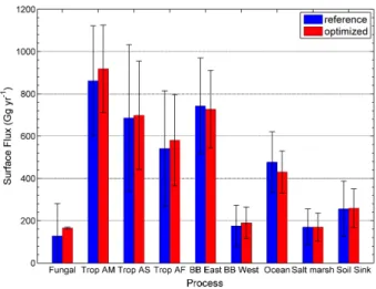
Fig. 11. Annual average CH3Cl surface flux magnitudes. Shown are the reference (blue bars) and optimized (red bars) values with their 1σ error bars (black). The errors on the references are the assumed a priori inversion uncertainties of±30% to±50%.
Northern Hemisphere in spring, and decreased the BB East-ern emission peak in the SouthEast-ern Hemisphere in spring. The inversion also increased the BB Western emission peak in the Southern Hemisphere in spring.
Global ocean optimized emissions retain some of the sea-sonal variability seen in the reference, but with an overall re-duction. The highest emission rates occur during the spring, resulting from the combined effects of the high monthly mean wind speeds and sea surface temperatures (Lee-Taylor et al., 2001). Compared to the reference values, emissions from global salt marshes are deduced to have a weak semi-annual rather than a strong semi-annual cycle. Finally, the peak in the global soil sink shifts from August to September.
5.3.2 Average annual results
The inversion results are finally averaged over the entire pe-riod between 2000–2004 to illustrate the global budget of CH3Cl (Fig. 11 and Table 3). We have aggregated the
re-gional tropical plant and biomass burning emissions in Ta-ble 3; their individual regional fluxes are listed in TaTa-ble 4. The multi-year averages for the seasonal processes are de-rived by averaging the results shown in Fig. 6. The inversion has directly solved for the aseasonal fungal process emis-sions as multi-year average values. Figure 11 and Table 3 also include the optimized emission errors, which are al-ways less than the reference errors due to their reduction by the observations in the Kalman filter. For the seasonal pro-cesses, Eq. (3) has been extended to all months to determine the annual average errors. In Fig. 11, the aseasonal fungal uncertainty is taken from the last step of the Kalman filter. Note that the final error for the fungal emission estimate is much smaller than for the seasonal flux estimates. This is because the inversion solves the global fungal emission as a time-invariant variable over the entire period, thus allow-ing error reduction at every monthly time step. To provide a more realistic uncertainty estimate for the fungal emissions, we have multiplied the initial uncertainty estimate by the av-eraged percentage standard deviation reduction computed for the eight seasonal processes/regions to obtain the final error estimate shown in Table 3. The seasonal processes, in con-trast, have been solved as monthly fluxes which already add greater uncertainty to their five-year averages.
The inversion results indicate large CH3Cl emissions of
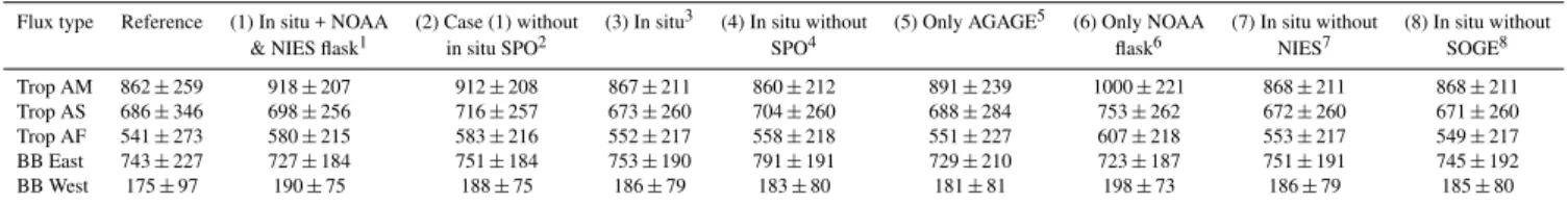
Table 4. Reference and optimally estimated five-year averaged surface fluxes and errors for emissions from tropical plants and biomass burning in Table 3.
Flux type Reference (1) In situ + NOAA (2) Case (1) without (3) In situ3 (4) In situ without (5) Only AGAGE5 (6) Only NOAA (7) In situ without (8) In situ without & NIES flask1 in situ SPO2 SPO4 flask6 NIES7 SOGE8
Trop AM 862±259 918±207 912±208 867±211 860±212 891±239 1000±221 868±211 868±211 Trop AS 686±346 698±256 716±257 673±260 704±260 688±284 753±262 672±260 671±260 Trop AF 541±273 580±215 583±216 552±217 558±218 551±227 607±218 553±217 549±217 BB East 743±227 727±184 751±184 753±190 791±191 729±210 723±187 751±191 745±192 BB West 175±97 190±75 188±75 186±79 183±80 181±81 198±73 186±79 185±80
1Using data from all in situ sites, the NIES HAT flask site, and the PSA, KUM, ALT, LEF, and HFM NOAA flask sites. This is the “best estimate” inversion case shown in the
figures.
2Inversion case (1) with NOAA in situ SPO site excluded.
3Using data from all in situ sites listed in Table 1.
4Inversion case (3) with NOAA in situ SPO site excluded.
5Using data only from AGAGE sites MHD, THD, RPB and CGO (the SMO measurements began after the time period of 2000–2005 addressed here).
6Using data from all 13 NOAA flask sites listed in Table 1.
7Inversion case (3) with NIES data excluded.
8Inversion case (3) with SOGE data excluded.
other source strengths are relatively small, and their per-centages are 11±2% for the oceans, 4±3% for the fungi, 4±2% for the salt marshes, 4% for the industry/incineration, and 1% for the wetlands. The total global emissions are 4089±471 Gg yr−1in the best estimate (Case 1 in Table 3). Relative to their a priori magnitudes, the inversion increases global fungal emissions, increases emissions from tropical plants and the western biomass burning source, and slightly reduces the global oceanic source and the eastern biomass burning source. The optimized global salt marsh emissions and soil sink show little change from their a priori values.
We also tested the sensitivity of the inversion results to 7 other alternative combinations of the observations used in the Kalman filter (Table 3). In general the inversion results in the 7 alternative cases studied agree within their errors with the results from the best estimate (Case 1), in part because of the consistency of the measurements from the different networks when placed on a common calibration scale.
The forward model has been run with the final optimal emission estimates, and the predicted mole fractions have been compared with the measurements. Figure 12 shows the residuals between the optimized and observed monthly mean mole fractions, compared to the residuals between the refer-ence and observed monthly mean mole fractions at each ob-serving site. The optimization lowers the residuals at many but not all of the sites. These differences are caused by a combination of the sensitivity of each site to the emitting re-gions and the precision and frequency of the measurements at the site. The average root-mean-square difference between the observed mole fractions and those calculated in the model run using the reference emissions is 31 ppt and this differ-ence is lowered to 24 ppt using the model run with optimized emissions.
6 Summary and discussion
In this paper we solved for monthly, annual, and interannual surface fluxes for the various source and sink categories of atmospheric methyl chloride during 2000–2004 using mea-surements from the AGAGE, NOAA/ESRL, SOGE, and NIES sampling networks, the MATCH 3-D global chemical transport model, and a Kalman filter with monthly pulses. The state vector in the Kalman filter includes scaling factors which multiply maps of the a priori estimates of each source and sink at monthly time resolution. The final optimally esti-mated sources and sink were used as input for a forward run of the MATCH model to test the inversion results.
Large CH3Cl emissions of 2200±390 Gg yr−1 are
esti-mated for tropical plants, which confirms the suggestion of Yokouchi et al. (2002) that tropical plants are the largest global source of CH3Cl. Relative to the a priori estimates,
the inversion estimates indicate increases in global fungal and tropical plant emissions, and reductions in global ocean emissions. Our revised budget indicates that a substantial fraction of the CH3Cl sources reside in the tropics and
sub-tropics (Fig. 13). Of our 20 independent observing sites, only 5 are tropical or sub-tropical (Barbados, Samoa, Hateruma, Mauna Loa, Mauna Kea), which implies the need for more tropical (preferably in situ) continuous observing sites in or-der to improve our unor-derstanding of the magnitudes and vari-abilities of the dominant tropical sources. Future inversions could also utilize short-term aircraft campaign data (e.g., Blake et al., 1996).
Regarding the temporal variability of the deduced fluxes, the inversion generally implies greater seasonal oscillations of the natural sources and sink of CH3Cl compared to the
Fig. 12. Residuals between the optimized and observed monthly mean mole fractions of CH3Cl (red lines), compared to the residuals between the reference and observed monthly mean mole fractions (blue lines) at each observing site.
Fig. 13. A posteriori annual average distribution of combined CH3Cl surface fluxes from the estimated sources and sink, the con-stant industrial source, and the annual average wetland emissions.
1997/1998 El Ni˜no, the global land precipitation appeared unusually low during this time period. There is evidence that the unusually dry land conditions have led to a strong NPP decrease, which can be expected to have caused a decrease in emissions of CH3Cl from tropical plants. The
anoma-lously dry and hot climate may also have led to increased insect damage to vegetation and they have increased the sus-ceptibility of the biomass to large-scale burning, leading to an increase in global biomass burning emissions of CH3Cl.
Furthermore, decreased organic matter content and microbial activity in soils associated with the dry conditions may be the reason for a reduction in global in-soil consumption.
Possi-ble future climate change involving increasingly dry and hot summers may lead to increased occurrence of reductions in emissions from the tropical biosphere and in uptake by soils, and increases in emissions from salt marshes and biomass burning. Therefore future CH3Cl levels will probably be
dependent on climate change and will contribute to the fu-ture trend in stratospheric chlorine. Fufu-ture studies involving coupled climate change/climate dependent CH3Cl emissions
may be necessary to more precisely predict global ozone re-covery over the next 50 years.
Our inversions for the interannual variability of different source or sink categories of CH3Cl are unavoidably affected
by the uncertainties in other model parameters which were not included in the inversions. We have used interannually varying meteorological data from observed meteorological reanalyses to minimize the uncertainty caused by transport, because interannual variations of transport can strongly af-fect calculated mole fractions (Chen and Prinn, 2005). An-other uncertainty originates from interannual variability of OH concentrations. In the inversions we used annually re-peating OH fields. A change of a few percent in the global average OH concentrations in the period 2000–2004 would cause an uncertainty of the same magnitude in the total de-duced sources which is well within the errors of our emission estimates.
to justify alternative distributions. Note also that we use monthly average measurements that omit obvious large pol-lution events in our inversions. Hence, our aggregate regional emissions are not biased by errors in the distribution of emis-sions at grid points close enough to the observing stations to produce these pollution events.
Finally, although the inverse modeling approach can be used to quantitatively estimate the magnitudes of sources and sinks of CH3Cl, field and laboratory experiments are still
necessary to improve the understanding of the mechanisms for the biochemical processes that control its natural sources and sinks. Keppler et al. (2005) studied the abiotic methy-lation of chloride in terrestrial ecosystems, and calculated a global soil sink for CH3Cl of more than 1000 Gg yr−1, which
is much larger than our estimate thus inviting further process studies of this sink.
Appendix A
The Kalman filter
The Kalman filter has been used in a number of studies to estimate the atmospheric lifetime or global sources of chlorofluorocarbons (e.g., Cunnold et al., 1983; Hartley and Prinn, 1993; Mahowald et al, 1997b; Mulquiney and Norton, 1998; Prinn et al., 2000) and other trace gases (e.g., Xiao et al., 2007, 2010; Xiao, 2008). It processes all available mea-surements, accounting for their precision, to estimate the cur-rent values of the quantities of interest (the states), with use of: (1) knowledge of the system and measurement instrument dynamics; (2) the statistical description of the system errors, measurement noise, and uncertainty in the dynamics models; and (3) any available information about the initial conditions of the state variables of interest. The covariance matrix,P, of the error in the state estimate is also computed.
An introduction to the Kalman filter for application to esti-mating sources and sinks for atmospheric trace gases can be found in Prinn (2000), in which the Kalman filter recursion from timek−1 to timekconsists of two steps:
Step 1: state vector extrapolation
xfk=Mk−1xak−1 (A1)
Pfk=Mk−1Pak−1M T
k−1+Qk−1 (A2)
Step 2: state vector improvement
xak=xfk+Kk(yok−Hkxfk) (A3)
Pak=Pfk−KkHkPfk (A4)
where
Kk=PfkHTk(HkPfkHTk+Rk)−1 (A5)
is the Kalman gain matrix. In the equationsxk is the state
vector (the superscripts f and a refer to the values before (forecast) and after (analysis) the use of thek-th measure-mentyok). Rk is the associated measurement error
covari-ance matrix, andHkis the sensitivity matrix that relates mole
fraction changes at observation sites to emission changes at different regions. The matricesQandMare discussed later. Here we use the unit pulse method of Chen and Prinn (2006), in which we adapt the Kalman filter to estimate CH3Cl surface fluxes from different sources and sinks at
monthly time resolution on regional or global scales. Sup-pose we havenastime invariant (aseasonal) andnsseasonally
varying surface flux variables forNyears. The full state vec-tor is therefore composed ofnas+N×12×nselements. This
is a large number and imposes a large demand on computer time. However, because the global horizontal mixing time in the model is about 1 year, an observation cannot mean-ingfully provide information about monthly fluxes that occur more than one year before the observation (Chen and Prinn, 2006). Hence, it is a good approximation to use a specific monthly observation at timekto deduce not all but only those monthly fluxes from timekback to timek−T (whereT=11 months). The resultant down-sized state vector was given earlier in Eq. (1):
xk=
Xask Xsk Xsk−1
...
Xsk−T
(A6)
where Xask is a subvector containing all the nas aseasonal
flux variables, andXsk is a subvector containing all thens
monthly/seasonal flux variables at timek. Notice thatXsk−T
contains the “oldest” seasonal fluxes that the observationyok
can provide meaningful information about. Therefore it con-tains the final, optimized solution for fluxes at timek−T
and is then removed from the state vector before a new ob-servation yok+1 is included. To achieve this removal, Chen and Prinn (2006) borrow the mathematics (but not the un-derlying concepts) used for extrapolation of the state vector and its error covariance matrix (Eqs. A1 and A2). A constant transition matrix is used with the following form:
M=
Inas 0 0 0 0
0 0 0 0 0
0 Ins 0 0 0
0 0 Ins 0 0
... ... ... ... ...
0 0 0 Ins 0
(A7)
whereInas andIns represent square identity sub-matrices of
sizesnasandnscorresponding tonasaseasonal fluxes andns
all zero elements. The transition matrix operates on the state vector as follows:
⎥ ⎥ ⎥ ⎥ ⎥ ⎥ ⎥ ⎥ ⎦ ⎤ ⎢ ⎢ ⎢ ⎢ ⎢ ⎢ ⎢ ⎢ ⎣ ⎡ • ⎥ ⎥ ⎥ ⎥ ⎥ ⎥ ⎥ ⎥ ⎦ ⎤ ⎢ ⎢ ⎢ ⎢ ⎢ ⎢ ⎢ ⎢ ⎣ ⎡ + s s 1 s 1 s as 0 0 0 0 0 0 0 0 0 0 0 0 0 0 0 0 0 0 0 0 0 s s s as k-T k-T k-k k n n n n X X ... X X X ... ... ... ... ... I I I I (A8) ⎥ ⎥ ⎥ ⎥ ⎥ ⎥ ⎥ ⎥ ⎦ ⎤ ⎢ ⎢ ⎢ ⎢ ⎢ ⎢ ⎢ ⎢ ⎣ ⎡ = + s 1 s 1 s as 0 k-T k-k k X ... X X X
Xk-Ts = optimized fluxes
Multiplying xk by M not only removes Xsk−T which is
saved as the final, optimized solution, but also introduces a newXsk+1 whose initial guess is its (unity) a priori value. For the aseasonal components, the transition matrix retains the previous values, which is consistent with the estimation of time invariant fluxes over all time steps.
Operation ofMon the error covariance matrixPakofxkhas
similar effects as onxk by removing the error covariances of Xsk−T, but it introduces zeros for the initial error covariances ofXsk+1to be estimated. This problem is solved by including the matrixQkin the following form:
Qk=
0 0 0 0 0
0 E ekeTk
0 0 0
0 0 0 0 0
0 0 0 0 0
... ... ... ... ...
0 0 0 0 0
(A9)
where E[ekeTk]represents the choice of the initial error
co-variances associated with the new seasonal flux adjustments (Xsk+1).
Acknowledgements. We thank David Kicklighter and Julia Lee-Taylor for sharing their research results as the a priori inputs into this work. We also thank the two anonymous reviewers for their constructive comments that improved the manuscript. The inversions and the AGAGE measurements were supported by a variety of sources, including: NASA grants NNX07AE89G, NAG5-12669 and NAG5-12099 (and associated NCCS computer support), and NSF grant ATM-0120468 (and associated NCAR computer support) to MIT; NASA grants NNX07AF09G and NNX07AE87G, to SIO; the Australian Bureau of Meteorology and CSIRO-MAR; and DEFRA grants EPG 1/1/159, CPEG 24, and GA01081 to Bristol University. The HATS flask and HATS high frequency in situ measurements were supported by NOAA-ESRL. Financial support for the Zeppelin measurements is acknowledged from the Norwegian Pollution Control Authority (SFT). NIES measurements were supported by the Global Environment Research Fund (Ministry of the Environment of Japan).
Edited by: P. Monks
References
Ayres, M. P. and Lombardero, M. J.: Assessing the consequences of global change for forest disturbance from herbivores and pathogens, Sci. Total Environ., 262, 263–286, 2000.
Balzter, H., Gerard, F. F., George, C. T., Rowland, C. S., Jupp, T. E., McCallum, I., Shvidenko, A., Nilsson, S., Sukhinin, A., Onuchin, A., and Schmullius, C.: Impact of the Arctic oscillation pattern on interannual forest fire variability in Central Siberia, Geophys. Res. Lett., 32, L14709, doi:10.1029/2005GL022526, 2005.
Blake, N. J., Blake, D. R., Sive, B. C., Chen, T.-Y., Rowland, F. S., Collins Jr., J. E., Sachse, G. W., and Anderson, B. E.: Biomass burning emissions and vertical distribution of atmo-spheric methyl halides and other reduced carbon gases in the South Atlantic region, J. Geophys. Res., 101, D19, 24151-24164, 1996.
Butler, J. H., Battle, M., Bender, M., Montzka, S. A., Clarke, A. D., Saltzman, E. S., Sucher, C., Severinghaus, J., and Elkins, J. W.: A twentieth century record of atmospheric halocarbons in polar firn air, Nature, 399, 749–755, 1999.
Chen, Y.-H. and Prinn, R. G.: Atmospheric modeling of high-and low-frequency methane observations: Importance of in-terannually varying transport, J. Geophys. Res., 110, D10303, doi:10.1029/2004JD005542, 2005.
Chen, Y.-H. and Prinn, R. G.: Estimation of atmospheric methane emissions between 1996 and 2001 using a three-dimensional global chemical transport model, J. Geophys. Res., 111, D10307, doi:10.1029/2005JD006058, 2006.
Ciais, P., Reichstein, M., Viovy, N., Granier, A., Og´ee, J., Allard, V., Aubinet, M., Buchmann, N., Bernhofer, C., Carrara, A., Cheval-lier, F., Noblet, N. D., Friend, A. D., Friedlingstein, P., Gr¨unwald, T., Heinesch, B., Keronen, P., Knohl, A., Krinner, G., Loustau, D., Manca, G., Matteucci, G., Miglietta, F., Ourcival, J. M., Pa-pale, D., Pilegaard, K., Rambal, S., Seufert, G., Soussana, J. F., Sanz, M. J., Schulze, E. D., Vesala, T., and Valentini, R.: Europe-wide reduction in primary productivity caused by the heat and drought in 2003, Nature, 437, 529–533, 2005.
Clerbaux, C. and Cunnold, D. M.: Chapter 1 in: Scientific Assess-ment of Ozone Depletion: 2006, Global Ozone Research and Monitoring Project Report No. 50, Geneva, Nairobi; Washing-ton, DC, Brussells: NOAA, NASA, UNEP, WMO, EC., 1.1– 1.63, 2006.
Cleveland, C. C., Holland, E. A., and Neff, J. C.: Temperature reg-ulation of soil respiration in an alpine tundra ecosystem, paper presented at the Front Range Branch Annual Meeting, Am. Geo-phys. Union, Golden, Colo., 8–10 February, 1993.
Cox, M. L., Sturrock, G. A., Fraser, P. J., Siems, S. T., Krummel, P. B., and O’Doherty, S.: Regional sources of methyl chloride, chloroform and dichloromethane identified from AGAGE obser-vations at Cape Grim, Tasmania, 1998–2000, J. Atmos. Chem., 45, 79–99, 2003.
Cox, M. L., Fraser, P. J., Sturrock, G. A., Siems, S. T., and Porter, L. W.: Terrestrial sources and sinks of halomethanes near Cape Grim, Tasmania, Atmos. Environ., 38(23), 3839–3852, 2004. Cunnold, D. M., Prinn, R. G., Rasmussen, R. A., Simmonds, P.
Graedel, T. E. and Keene, W. C.: The tropospheric budget of reac-tive chlorine, Global Biogeochem. Cy., 9, 47–77, 1995. Graedel, T. E. and Keene, W. C.: The budget and cycle of Earth’s
natural chlorine, Pure Appl. Chem., 68, 1687–1689, 1996. Graedel, T. E. and Keene, W. C.: Preface, J. Geophys. Res.,
104(D7), 8331–8332, 1999.
Guenther, A., C. Hewitt, N., Erickson, D., Fall, R., Geron, C., Graedel, T., Harley, P., Klinger, L., Lerdau, M., McKay, W. A., Pierce, T., Scholes, B., Steinbrecher, R., Tallamraju, R., Tay-lor, J., and Zimmerman, P.: A global model of natural volatile organic compound emissions, J. Geophys. Res., 100(D5), 8873– 8892, 1995.
Hamilton, J. T. G., McRoberts, W. C., Keppler, F., Kalin, R. M., and Harper, D. B.: Chloride methylation by plant pectin: An efficient environmentally significant process, Science, 301, 206– 209, 2003.
Hao, W. M. and Liu, M.-H.: Spatial and temporal distribution of tropical biomass burning, Global Biogeochem. Cy., 8(4), 495– 503, 1994.
Hartley, D. E. and Prinn, R. G.: On the feasibility of determining surface emissions of trace gases using an inverse method in a three-dimensional chemical transport model, J. Geophys. Res., 98, 5183–5198, 1993.
Holland, E. A., Townsend, A. R., and Vitousek, P. M.: Variability in temperature regulation of CO2fluxes and N mineralization from five Hawaiian soils: Implications for a changing climate, Global Change Biol., 1, 115–123, 1995.
J¨ockel, P.: Cosmogenic14CO as tracer for atmospheric chemistry and transport, Rpertus Carola University of Heidelberg, Heidel-berg, 2000.
Keene, W. C., Khalil, M. A. K., Erickson III, D. J., McCulloch, A., Graedel, T. E., Lobert, J. M., Aucott, M. L., Gong, S. L., Harper, D. B., Kleiman, G., Midgley, P., Moore, R. M., Seuzaret, C., Sturges, W. T., Benkovitz, C. M., Koropalov, V., Barrie, L. A., and Li, Y. F.: Composite global emissions of reactive chlo-rine from anthropogenic and natural sources: Reactive Chlochlo-rine Emissions Inventory, J. Geophys. Res., 104(D7), 8429–8440, 1999.
Keppler, F., Harper, D. B., R¨ockmann, T., Moore, R. M., and Hamil-ton, J. T. G.: New insight into the atmospheric chloromethane budget gained using stable carbon isotope ratios, Atmos. Chem. Phys., 5, 2403–2411, doi:10.5194/acp-5-2403-2005, 2005. Khalil, M. A. K.: Reactive chlorine compounds in the atmosphere,
in: Reactive Halogen Compounds in the Atmosphere, edited by: Fabian, P. and Singh, O. N., Springer-Verlag, Berlin, Heidelburg New York, 45–79, 1999.
Khalil, M. A. K. and Rasmussen, R. A.: Atmospheric methyl chlo-ride, Atmos. Environ., 33, 1305–1321, 1999.
Khalil, M. A. K., Moore, R. M., Harper, D. B., Lobert, J. M., Er-ickson, D. J., Koropalov, V., Sturges, W. T., and Keene, W. C.: Natural emissions of chlorine-containing gases: Reactive Chlo-rine Emission Inventory, J. Geophys. Res., 104(D7), 8333–8346, 1999.
Knorr, W., Gobron, N., Scholze, M., Kaminski, T., Schnur, R., and Pinty, B.: Impact of terrestrial biosphere carbon exchanges on the anomalous CO2increase in 2002–2003, Geophys. Res. Lett., 34, L09703, doi:10.1029/2006GL029019, 2007.
Kobak, K. I., Turchinovich, I. Y., Kondrasheva, N. Y., Schulze, E. D., Schulze, W., Koch, H., and Vygodskaya, N. N.: Vulnerability
and adaptation of the larch forest in eastern Siberia to climate change, Water Air Soil Pollut., 92, 119–127, 1996.
Krummel, P. B.: the AGAGE team and respective participating lab-oratory investigators: Inter-comparison of AGAGE trace gases with other laboratories: ftp://gaspublic:gaspublic@ftp.dar.csiro. au/agage/, last access: 27 January 2009.
Lawrence, M. G., Crutzen, P. J., Rasch, P. J., Eaton, B. E., and Mahowald, N. M.: A model for studies of tropospheric photo-chemistry: Description, global distributions, and evaluation, J. Geophys. Res., 104(D21), 26245–26277, 1999.
Lee-Taylor, J. M., Doney, S. C., Brasseur, G. P., and M¨uller, J.-F.: A global three-dimensional atmosphere-ocean model of methyl bromide distributions, J. Geophys. Res., 103(D13), 16039– 16057, 1998.
Lee-Taylor, J. M., Brasseur, G. P., and Yokouchi, Y.: A preliminary three-dimensional global model study of atmospheric methyl chloride distributions, J. Geophys. Res., 106(D24), 34221– 34233, 2001.
Lobert, J. M., Keene, W. C., Logan, J. A., and Yevich, R.: Global chlorine emissions from biomass burning: Reactive Chlorine Emissions Inventory, J. Geophys. Res., 104(D7), 8373–8389, 1999.
Lucas, D. D. and Prinn, R. G.: Sensitivities of gas-phase dimethyl-sulfide oxidation products to the assumed mechanisms in a chemical transport model, J. Geophys. Res., 110, D21312, doi:10.1029/2004JD005386, 2005.
Lyon, B: The strength of El Ni˜no and the spatial ex-tent of tropical drought, Geophys. Res. Lett., 31, L21204, doi:10.1029/2004GL020901, 2004.
Mahowald, N. M.: Development of a 3-dimensional chemical trans-port model based on observed winds and use in inverse modeling of the source of CCl3F, PhD thesis, MIT, Cambridge, 1996. Mahowald, N. M., Rasch, P. J., Eaton, B. E., Whittlestone, S., and
Prinn, R. G.: Transport of222radon to the remote troposphere using the Model of Atmospheric Transport and Chemistry and assimilated winds from ECMWF and the National Center for Environmental Prediction/NCAR, J. Geophys. Res., 102(D23), 28139–28151, 1997a.
Mahowald, N. M., Prinn, R. G., and Rasch, P. J.: Deducing CCl3F emissions using an inverse method and chemical transport mod-els with assimilated winds, J. Geophys. Res., 102(D23), 28153– 28168, 1997b.
McCulloch, A., Aucott, M. L., Benkovitz, C. M., Graedel, T. E., Kleiman, G., Midgley, P. M., and Li, Y. F.: Global emissions of hydrogen chloride and chloromethane from coal combustion, in-cineration and industrial activities: Reactive Chlorine Emissions Inventory, J. Geophys. Res., 104(D7), 8391–8403, 1999. McGuire, A. D., Sitch, S., Clein, J. S., Dargaville, R., Esser, G.,
Foley, J., Heimann, M., Joos, F., Kaplan, J., Kicklighter, D. W., Meier, R. A., Melillo, J. M., Moore III, B., Prentice, I. C., Ra-mankutty, N., Reichenau, T., Schloss, A., Tian, H., Williams, L. J., and Wittenberg, U.: Carbon balance of the terrestrial biosphere in the twentieth century: analyses of CO2, climate and land use effects with four process-based ecosystem models, Global Biogeochem. Cy., 15(1), 183–206, 2001.