Abstract
In this study, vibration behavior of orthotropic cylindrical shells with variable thickness is investigated. Based on linear shell theory and applying energy method and using spline functions, free vibration relations are derived for shell with variable thickness and curvature. Frequency parameter and mode shapes are found after solving the frequency Eigenvalue equation. Effects of variable thickness along axial and circumferential directions of the shell on its frequency parameter are studied and compared against each other. Shell thickness is assumed to be varied in a parabolic profile along both directions. Also, frequency parameters for both circular and parabolic curvatures along circumferential direction are inves-tigated and results are compared together. In addition, effect of variable thickness on the mode shapes is studied.
Keywords
Cylindrical shell, Parabolic curvature, Variable thickness, Natural frequency, Spline function, Discrete method.
Free Vibration Analysis of Orthtropic Thin Cylindrical Shells
with Variable Thickness by Using Spline Functions
1 INTRODUCTION
Cylindrical (open) shells with either circular or noncircular profiles have been widely used in recent years, as structural elements within marine, civil, aerospace, and petrochemical industries. In addi-tion, because of inherent difficulties in assembly of shells with circular profile, noncircular profile is preferred in constructing cylindrical shells. Vibration behavior of cylindrical shells with circular profile is different than that of cylindrical shells with noncircular profile.
Variation of the thickness in a cylindrical shell leads to decrease of its structural weight besides reducing cost of needed materials. Moreover, natural frequency of the shell changes as a result of its variable thickness. Therefore, vibration analysis of the shells with variable thickness has attracted the attention of many researchers in recent years.
Pouria Bahrami Ataabadia Mohammad Reza Khedmati* a Mostafa Bahrami Ataabadib
a Department of Marine Technology,
Amirkabir University of Technology, 424 Hafez Avenue, Tehran 15916-34311, Iran
b Department of Engineering and
Build-ing, National Iranian Oil Company, Boushehr, 3rd Pars 75391-154, Iran
*Author email: [email protected]
Latin American Journal of Solids and Structures 12 (2014) 2099-2121
Zhang et al. (2001) and Pellicano (2007) studied vibration behavior of the shells incorporating
circular profile and uniform thickness. A few other researchers have also studied vibration response of noncircular shells, among them are Srinivasan and Bobby (1976), Cheung and Cheung (1972) and Yamada et al. (1999).
Vibration response of flat plates with variable thickness has also been addressed by Huang et al.
(2005, 2007), Ashour (2001), Sakiyama and Huang (1998), Grigorenko et al. (2008). On the other
hand, Sivadas and Ganesan (1991), Zhang and Xiang (2006), Duan and Koh (2008) investigated vibration response of the closed shells having circular profiles and variable thickness. Their investi-gations were limited to the effects of variable thickness in one direction (either axial or circumferen-tial) on vibration behavior of the shells. Later, Grigorenko and Parkhomenko (2011) studied free vibration of shallow shells having parabolically-variable thickness with the aid of spline-collocation approach. The effects of variable thickness on the vibration behavior of closed elliptical cylindrical shells and closed oval cylindrical shells have been studied by Suzuki and Leissa (1985) and Khalifa (2011), respectively.
Open parabolic cylindrical shell with variable thickness is considered as the main geometry in the present study. As it was shown, very few research works have been performed on such struc-tures. In addition, vibration response of parabolic cylindrical shells and circular cylindrical shells are compared against each other’s. As it was mentioned earlier, most of the previous works studied the effects of thickness variation in one direction on the vibration response of the shells. Therefore, a thorough study on the effects of direction of thickness variation on the vibration response of a shell is lacked herein. Present work is aimed at study of vibration response for both parabolic shells and circular shells having variable thickness in either axial direction or circumferential direction. On the other hand, analytical solutions cannot be simply reached for assessment of vibration re-sponse of the shells when both radius and thickness are subjected to variation. Thus, numerical approaches as well as approximate methods may be used to investigate the vibration response of these types of the shells. Techniques based on spline functions are among numerical methods that are useful in solving structural problems. In the present work, a relatively simple discrete method incorporating spline functions introduced already by Cheng and Chuang (1990) and Cheng et al.
Latin American Journal of Solids and Structures 11 (2014) 2099-2121 2 THEORY AND FORMULATIONS
Since thickness of the shell is small compared to its other dimensions, the shell is regarded to be thin. Consequently, classical shell theory based on Kirchhoff–Love assumptions is used to extract governing equations.
2.1 Geometric formulation
The main geometry under consideration in this work is a cylindrical shell with an either circular or parabolic profile. Both circular and parabolic profiles can be defined by two parameters including camber (C) and span (b), Figure 1. Geometrical relations for circular and parabolic profiles are given in Table 1.
(a) (b)
Figure 1: (a) circular profile and (b) parabolic profile.
Figure 2 shows a shell with a parabolic profile in the curvilinear coordinate system (xsz). z-axis is perpendicular to the middle surface of shell defined by x-s plane. x-axis is along axis of the cylinder, while the s-axis is along circumference of the cylinder. Displacement functions along x-axis, s-axis and z-axis are respectively represented by U(x,s), V(x,s) and W(x,s). Lame’s parameters for this type of shell in the curvilinear coordinate system are equal to one according to Soedel (1993).
Latin American Journal of Solids and Structures 12 (2014) 2099-2121
2.2.Displacement functions
Displacement functions for the middle surface of the shell are introduced by cubic and fifth-order B-spline functions as below.
( )
( )
( ) { } (
)
( )
( )
( ) { } (
)
( )
φ( )
φ( ) { } (
)
U x, s x s A sin t e
V x, s s B sin t e
W x, s x s C sin t e
x
f f
f f
ê ú ê ú
=ë ûÄë û +
ê ú ê ú
= ë ûÄë û +
ê ú ê ú
=ë ûÄë û +
(1)
Row matricesêëf
( )
x úûandêëj( )
x úûare cubic B-spline and fifth-order B-spline matrices, respectively. Column matrices{ }
A ,{ }
B and{ }
C are unknown coefficients of the displacement functions in Equa-tion 1. Also, N is the number of divisions along x or s axes. The operatorÄis the ‘Kronecker prod-uct’ of the matrices. Formulations of row matrices and also column matrices are given below( )
( )
( ) ( )
( )
( ) ( )
( )
( )
( )
( )
( ) ( )
( )
φ
1 0 1 N 1 N N 1 N 3
2 1 0 N N 1 N 2 N 5
x x x x x x x
x x x x x x x
f f - f f f - f f +
+
- - + + +
é ù
ê ú = ê ¼¼ ú
ë û ë û
é ù
ê ú = ê ¼¼ ú
ë û ë û
{ }
{
} { }
{ } {
}
( )
{ }
{ }
{ }
{ }
{
} { }
{
} {
}
( )
{ }
T T T T T
1 0 N N 1
N 3 T
i i1 i2 i3 iN
T T T T T
2 1 N 1 N 2
N 5 T
i i1 i2 i3 iN
A a a a a
a a a a a , i 1, 0,1, N 1 A
C c c c c
c c c c c , i 2, 1
,
N 2
s
, 0,
B i same as
- + é ù
+ ë û
- - + + é ù
+ ë û
é ù
=ê ¼¼ ú
ë û
é ù
= êë ¼¼ úû = - ¼ +
é ù
= êë ¼¼ úû
é ù
=êë ¼¼ úû = - - ¼ +
(2)
Standard cubic spline is expressed as
( )
(
)
(
)
(
)
(
)
(
)
(
)
φ
3
3 3
3 3
3
3
2 x x 2, 1
2 x 4 1 x x 1, 0
1
x 2 x 4 1 x x 0,1
6
2 x x 1, 2
0 x 2
ìïï + Î - -é ù
ë û
ïï
ï é ù
ï + - + Î
-ï ë û
ïï
= íï - - - Îéë ùû
ïï
ï - Îé ù
ï ë û
ïï
ï >
ïî
(3)
According to Cheng et al. (1987), cubic B-spline functions (B3) for N equal divisions (N>4) are
φ
φ φ
φ φ φ φ φ
φ
i 3
1 3 N 2 3
0 3 3 N 1 3 3 3
1 3
x
i , i 3, 4, 5 , N 3 h
x x
1 N 2
h h
x x x 1 x x
4 1 N 1 N N 1
h h h 2 h h
x 1 h
f
f f
f f
f
-
-æ ö÷
ç ÷
= çççè - ÷÷ = ¼
-ø
æ ö÷ æ ö÷
ç ÷ ç ÷
= ççç + ÷÷ = ççç - + ÷÷
è ø è ø
æ ö÷ æ ö÷ æ ö÷ æ ö÷ æ ö÷
ç ÷ ç ÷ ç ÷ ç ÷ ç ÷
= çè øçç ÷÷- èççç + ÷ø÷ = èççç - + ÷ø÷- èççç - ÷ø÷+ çèçç - - ÷÷ø æç
= ç
-è φ φ φ φ
φ φ
3 3 N 3 3
2 3 N 1 3
1 x x x x
1 N 4 N 1
2 h h h h
x x
2 N 1
h f h
f
f +
ö æ ö æ ö æ ö æ ö
÷ ç ÷ ç ÷ ç ÷ ç ÷
÷- ç ÷+ ç + ÷ = ç - ÷- ç - - ÷
÷ ÷ ÷ ÷ ÷
ç ÷ ç ÷ ç ÷ ç ÷ ç ÷
ç ø çè ø çè ø çè ø çè ø
æ ö÷ æ ö÷
ç ÷ ç ÷
= ççç - ÷÷ = ççç - - ÷÷
è ø è ø
Latin American Journal of Solids and Structures 11 (2014) 2099-2121 Expression for the standard fifth-order spline is
(
)
(
)
(
)
(
)
(
)
(
)
(
)
(
)
(
)
(
)
(
)
(
)
φ
5
5 5
5 5 5
5 5 5
5
5 5
5
3 x x 3, 2
3 x 6 2 x x 2, 1
3 x 6 2 x 15 1 x x 1, 0
1
3 x 6 2 x 15 1 x x 0,1
120
3 x 6 2 x x 1, 2
3 x x 2, 3
0 x 3
ìï + Î - -é ù
ï ë û
ïï
ï é ù
ï + - + Î
-ï ë û
ïï
ï + - + + + Î -é ù
ï ë û
ïïï
= íï - - - + - Î éë ùû
ïï
ï - - - Îé ù
ï ë û
ïï
ï - Îé ù
ï ë û
ïï
ï >
ïïî
(5)
Again, according to Cheng et al. (1987), fifth-order B-spline functions (B5) for N equal divisions
(N>6) are
φ
φ
φ φ
α φ α φ φ
α φ α φ φ
i 5
2 5
1 5 5
0 11 5 12 5 5
1 21 5 22 5 5
x
i , i 4, 5, 6 N 4
h x
2 h
x x
1 26 2
h h
x x x
2 1
h h h
x x x
1
h h
-æ ö÷
ç
= çç - ÷÷÷ = ¼
-è ø
æ ö÷
ç = çç + ÷÷÷
è ø
æ ö÷ æ ö÷
ç ç
= çç + ÷÷÷- çç + ÷÷÷
è ø è ø
æ ö÷ æ ö÷ æ ö÷
ç ç ç
= çç + ÷÷÷+ çç + ÷÷÷+ çç ÷÷÷
è ø è ø è ø
æ ö÷ æ ö÷
ç ç
= çç + ÷÷÷+ çç ÷÷÷+
è ø è ø
α φ α φ φ
φ
φ
φ φ φ
φ
2 31 5 32 5 5
3 5
N 3 5
N 2 31 5 32 5 5
N 1 21 5
1 h
x x x
2 2
h h h
x 3 h
x
N 3
h
x x x
N 2 N N 2
h h h
x N h
-æ ö÷
ç - ÷
ç ÷
ç ÷
è ø
æ ö÷ æ ö÷ æ ö÷
ç ç ç
= çç + ÷÷÷+ çç ÷÷÷+ çç - ÷÷÷
è ø è ø è ø
æ ö÷
ç = çç - ÷÷÷
è ø
æ ö÷
ç
= çç - + ÷÷÷
è ø
æ ö÷ æ ö÷ æ ö÷
ç ç ç
= çç - + ÷÷÷+ çç - ÷÷÷+ çç - - ÷÷÷
è ø è ø è ø
= - φ φ
φ φ φ
φ φ
φ
22 5 5
N 11 5 12 5 5
N 1 5 5
N 2 5
x x
1 N N 1
h h
x x x
N 2 N 1 N
h h h
x x
N 1 26 N 2
h h
x
N 2
h
+ +
æ ö÷ æ ö÷ æ ö÷
ç - ÷+ ç - ÷+ ç - + ÷
ç ÷ ç ÷ ç ÷
ç ÷ ç ÷ ç ÷
è ø è ø è ø
æ ö÷ æ ö÷ æ ö÷
ç ç ç
= çç - - ÷÷÷+ çç - - ÷÷÷+ çç - ÷÷÷
è ø è ø è ø
æ ö÷ æ ö÷
ç ç
= çèç - - ø÷÷÷+ ççè - - ÷÷÷ø
æ ö÷
ç
= çç - - ÷÷÷
è ø
(6)
Latin American Journal of Solids and Structures 12 (2014) 2099-2121
α α
α α
α α
11 12 11 12
21 22 21 22 31 32 31 32
165 33
4 8
26 1
33 1 1
33
é - ù
é ù é ù ê ú
ê ú ê ú ê ú
ê ú =ê ú=ê - ú
ê ú ê ú ê ú
ê ú ê ú ê ú
ê ú ê ú ê - ú
ë û ë û ë û
And for ss boundary condition (simply supported edges at x=0, x=L)
α α
α α
α α
11 12 11 12 21 22 21 22
31 32 31 32
12 3
1 0
1 0
é ù é ù é - ù
ê ú ê ú ê ú
ê ú= ê ú= -ê ú
ê ú ê ú ê ú
ê ú ê ú ê- ú
ê ú ê ú ê ú
ë û ë û ë û
2.3 Mass and stiffness matrices
Extracted relations in this section are valid only for a shell with a general geometry.
2.3.1 Mass matrix
Kinetic energy of a shell with variable thickness can be expressed in the following form
(
2 2 2)
{ }
{ }
1 1
2 2
T shell shell shell
T =
òò
r t U +V +W dxds = d ëéMùû d (7)where, rshellis density, is thickness function of shell, U, V and W are displacement functions of the middle surface of shell. Also,
{ }
d = êéë{ } { } { }
A B C ùúûT, where{ }
A ,{ }
B and{ }
C are unknown coefficients of displacement functions.é ùë ûM is also mass matrix.After substituting the displacement functions (Equation 1) into the Equation 7 and taking nu-merical integration, the mass matrix is obtained by equation 8. This mass matrix is for a shell with variable thickness in x-direction. Through replacing x by s, the mass matrix for a shell with variable thickness in s-direction can be easily obtained.
(
)
(
)
(
)
ρ
tx s
shell tx s
tx s
F F 0 0
M 0 F F 0
0 0 H H
é Ä ù
ê ú
ê ú
é ù = ê Ä ú
ë û ê ú
Ä
ê ú
ë û
(8)
2.3.2 Stiffness matrix
Strain energy for a shell with a general geometry can be written as follows
{ }
{ }
{ }
{ }
1 1
2 2
T T
shell
U =
òò
e é ùë ûD e dxds = d é ùë ûK d (9)where, the strain vector is
Latin American Journal of Solids and Structures 11 (2014) 2099-2121 The components of strain vector are
1 1
1 1 2 1
2 2
2 1 2 2
2 1
12
1 2 2 1
1 1
1 1 1 1 2 2 2
2
2 2 2
A
1 U 1 W
V
A x A A s R
A
1 V 1 W
U
A s A A x R
A A V
A s A A s A
A
1 U 1 W 1 V 1 W
A x R A x A A s R A s
1 V 1 W
A s R A s
U
= + +
¶ 
= + +
¶ 
æ ö æ ö
¶ ç ÷÷ ¶ç ÷÷ = ççç ÷÷+ ççç ÷÷
¶ è ø ¶ è ø
é ¶ æç ¶ ö÷ ¶ æç ¶ öù÷
ê ÷ ÷ú
= -ê çç + ÷÷+ çç + ÷÷ú
ç ç
¶ è ¶ ø ¶ è ¶ ø
ë û
æ
¶ ç 
= - çç +
¶ è 
2
1 2 1 1
2
1 2 1 2
12 1 2 1 2 1 2 1 2 1 2
A
1 U 1 W
A A x R A x
A A A
1 1 W 1 W W 1 U 1
A A A s x A x s x s R A s A
W, U, V are displacement funct
A V
R A x A
é ö÷ ¶ æç ¶ öù÷
ê ÷÷+ çç + ÷÷ú
ê ç ÷ø ¶ çè ¶ ÷øú
ë û
é çæ ¶ ¶ ¶ ¶ ¶ ÷ö ¶æç ö÷ ¶ æç ö÷ù
ê ç-ç - + ÷÷+ çç ÷÷+ çç ÷÷ú
ê ç ÷÷ ç ÷ ç ÷ú
= -ê è ¶ ¶ ¶ ¶ ¶ ¶ ø ¶ è ø ¶ è øú
ê ú
ê ú
ë û
1
2
' 1 2
ions
R is radius of curvature along X axis
R is radius of curvature along S axis
A , A are Lame parameters
ìïï ïï ïï ïï ïï ïï ïï ïï ïï ïï ïï ïï ïï ïï íï ïï ïï ïï ïï ïï ïï ïï ïï ïï ïï ïï ï
-ïï
ïïî
Flexural rigidity of the shell is given as
( )
( )
( )
( )
( )
( )
( )
( )
( )
( )
11 12
21 22
66
11 12
21 22
66
B x, s B x, s 0 0 0 0
B x, s B x, s 0 0 0 0
0 0 B x, s 0 0 0
0 0 0 D x, s D x, s 0
0 0 0 D x, s D x, s 0
0 0 0 0 0 D x, s
D
é ù
ê ú
ê ú
ê ú
ê ú
ê ú
é ù = ê ú
ë û ê ú
ê ú
ê ú
ê ú
ê ú
ë û
( )
( )
( )
( )
( )
( )
( )
( )
( )
( )
( )
66
2 2
66 66 ,
, , , ,
1
, , , , ,
'
, ,
, ,
12 6
i i
ii ij j ii
ij i j
ij j ii ij
j ii
ii
E t x s E is elastic modulus
B x s D x s D x s
G is shear modulus
B x s B x s B G t x s t x s is thickness function
is poisson s ratio
B t x s B t x s
D x s D
J J J
J
J
ìïï = =
ïï
-ïï
ïï = =
íï ïï
ïï = =
ïïïî
Stiffness matrix is
11 12 13
T T T
21 22 23 21 12 31 13 32 23 31 32 33
k k k
K k k k , k k , k k , k k
k k k
é ù
ê ú
ê ú
é ù = ê ú = = =
ë û ê ú
ê ú
ë û
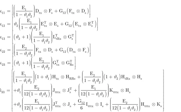
Latin American Journal of Solids and Structures 12 (2014) 2099-2121
(
)
(
)
(
)
(
)
111 tx s 12 tx s
1 2
T T
1
12 2 tx s 12 tx s
1 2
T T
1
13 2 tRx s
1 2 2
22 tx s 12 tx s
1 2
23 1
E
k D F G F D
1 E
k E E G E E
1
E
k 1 L G
1 E
k F D G D F
1 k J J J J J J J J J J J
éæç ö÷ ù
ê ÷ ú
=êçç ÷÷ + ú
ç
-è ø
ë û
é æç ö÷ ù
ê ÷ ú
= ê çç ÷÷ + ú
ç
-è ø
ë û
é æç ö÷ ù
ê ÷ ú
= ê + çç ÷÷ ú
ç
-è ø
ë û
éæç ö÷ ù
ê ÷ ú
=êççç ÷÷ + ú
Ä Ä Ä Ä Ä Ä -è ø ë û = Ä +
(
)
(
)
(
)
(
)
(
)
(
)
T T 2 tx Rs 1 2 1 21 tx RRs 2 tRx s
1 2 1 2
T
2 1
33 1 tttx s tttx s
1 2 1 2
1 2
1 2
E
1 G G
1
E E
1 H H 1 H H
1 1
E E
J J K H
12 1 12 1
E J 12 1 k J J J J
J J J J
J
J J J J
J
J J
é æç ö÷ ù
ê çç ÷÷ ú
ê ç -è ÷ø ú
ë û
æ ö÷ æ ö÷
ç ÷ + +ç ÷ +
ç ÷ ç ÷
ç ÷ ç ÷
ç - ç
-è ø è ø
æ ö÷ æ ö÷
ç ÷ ç ÷
ç ç
= + ç ÷÷ +ç ÷÷
÷ ÷
ç - ç
-è ø è ø
æ ö÷
ç ÷
ç
+ ç ÷÷÷
ç -è ø Ä Ä Ä Ä Ä
(
)
T 12 2
tttx s tttx s tttx s
1 2
G E
J I I H K
6 12 1 J J
é ù ê ú ê ú ê ú ê ú ê ú ê ú ê ú
ê æ ö ú
ê ç ÷÷ ú
ç
+ +
ê ç ÷÷ ú
ê çè - ÷ø ú
ë û
Ä Ä Ä
(10)
Some matrices are available in the list of the elements in the formulations of mass and stiffness matrices, which are called as spline matrices. Some of these spline matrices have been already de-rived by Cheng et al. (1987), while other spline matrices representing the effect of variable radius
and thickness are extracted herein. Formulations of all spline matrices are presented in Table 2 and Table 3.
( )
( )
L T x 0F =
ò
ëêf x û êú ëf x dxúû φ( )
( )
LT ' x
0
L =
ò
êë x ûú ëêêf x úúûdx φ( )
φ( )
LT
' '
x 0
I =
ò
êêë x ú êú êû ë x dxúúû( )
( )
φ L T x 0G =
ò
êë x úû êëf x úûdx( )
( )
LT
' '
x 0
D =
ò
êêëf x úúû ëêêf x úúûdx φ( )
φ( )
LT '' x
0
J =
ò
êë x úû êêë x úúûdx( )
( )
φ φ L T '' '' x 0K =
ò
êêë x û ëú êú ê x úûúdx φ( )
φ( )
LT x
0
H =
ò
êë x ú êû ë x dxúû( )
( )
LT ' x
0
E =
ò
ëêf x úû ëêêf x úúûdx( )
( )
φ L T ' x 0Z =
ò
êêë x ú êú ëû f x dxûú φ( )
φ( )
LT '' ' x
0
S =
ò
êêë x ú êú êû ë x dxúúûNote: Through replacing x by s in these relations, spline matrices in s direction can be obtained.
Table 2: Spline matrices used in this study and also the study of Cheng et al. (1987).
2.4 Frequency equation
Total potential energy for free vibration of a shell is expressed as follows
{ }
(
)
{ }
π
Π =2 éê T é ùK - 2é ùM ùú
ë û ë û
Latin American Journal of Solids and Structures 11 (2014) 2099-2121 Substituting mass and stiffness matrices into the above equation and using the Hamilton’s principle, following form of the frequency equation is obtained.
(
é ùK - 2é ùM)
{ }
=0ë û ë û (12)
Equation 12 is of eigenvalue type in which the eigenvalues represent the natural frequencies. Unknown coefficients of displacement functions create the eigenvectors. Solving the Equation 12 will result in the frequencies and corresponding mode shapes.
3 NUMERICAL EXAMPLES AND DISCUSSIONS
Based on derived formulations in the previous section, a code was written in the MATLAB envi-ronment in order to calculate the natural frequencies and also corresponding mode shapes.
3.1 Verification of present method
Accuracy of presented formulations is investigated in this section in order to demonstrate its ability to analyze free vibration of both parabolic and circular cylindrical shells with either uniform or var-iable thickness. A comparison between natural frequencies for a circular cylindrical shell having a uniform thickness as obtained by the present method and also by Srinivasan and Bobby (1976) is given in Table 4. It should be mentioned that Srinivasan and Bobby (1976) used Rayleigh–Ritz and matrix methods in their work. On the other hand, natural frequencies as obtained by the present method and the method developed by Cheung and Cheung (1972) are provided in Table 5 for a parabolic cylindrical shell with a constant thickness. Cheung and Cheung (1972) used strip method to extract relations for vibration analysis of a cylindrical shell with parabolic profile. In Table 6 results of the present method have been compared with those of Huang et al. (2005) who used
dis-( ) dis-( )
( )
L
T tx
0
F =
ò
t x êëf x ú êû ëf x dxúû φ( )
bT ' Rs
0
L =
ò
êë s úû ëêêf(s) dsúúû( ) ( )
φ LT ' tx
0
L =
ò
t x ëê x úû ëêêf(x) dxúúû( ) ( )
φ φ( )
L
T
3 ' '
tttx 0
I =
ò
t x ëêê x ú êú êû ë x dxúúû φ( )
( )
T bRs
s 0
s s
G ds
R f
ê ú ê ú
ë û ë û
=
ò
( ) ( )
φL
T tx
0
G =
ò
t x êë x ú êû ëf(x) dxúû( ) ( )
L
T
' '
tx 0
D =
ò
t x ëêêf x ú êú êû ëf(x) dxúúû φ( )
φ( )
Tb ''
Rs
s 0
s
J ds
R s
ê ú
ê ú
ë û
ê ú
ë û
=
ò
( ) ( )
φ φL
T
3 ''
tttx 0
J =
ò
t x êë x úû ëêê (x) dxúúû( )
( )
φ T φ
b
RRs 2
s 0
s s
H ds
R
ê ú ê ú
ë û ë û
=
ò
φ( )
φ( )
T b
Rs
s 0
s s
H ds
R
ê ú ê ú
ë û ë û
=
ò
( ) ( )
φ φ( )
L
T tx
0
H =
ò
t x êë x ú êû ë x dxúû( ) ( )
φ φ( )
L
T
3 '' ''
tttx 0
K =
ò
t x êëê x úúû êêë x úúûdx( ) ( )
( )
L
T ' tx
0
E =
ò
t x êëf x úû ëêêf x úûúdxNote: Through replacing x by s in matrices, spline matrices in s direction can be obtained.
Latin American Journal of Solids and Structures 12 (2014) 2099-2121
crete method in combination with Green’s function to obtain natural frequency solution for flat plates with variable thickness in one direction. Table 7 shows frequency parameters for a shallow shell with rectangular platform that its thickness varies parabolically in one direction (Grigorenko and Parkhomenko (2011)). Grigorenko and Parkhomenko (2011) obtained their solution method by using spline-collocation method.
Difference (%) Petyt as reported in Srinivasan
and Bobby (1976) Present work
Analysis Method Mesh Divisions
Mode
number 16 16 Re .[3]
Re .[3]
100
f f
w w
w
´
æ - ö÷
ç ÷
ç ÷
ç ÷÷
çè ø
Finite element Extended
Ray-leigh-Ritz 16 16´
14´14
12 12´
-0.68 870
870 876
879 882
1st
0.31 958
958 955
957 959
2nd
0.46 1288
1288 1282
1284 1297
3rd
-0.14 1363
1364 1366
1367 1369
4th
-0.20 1440
1440 1443
1444 1446
5th
2 2 2
s
E1.0e7lb in ,R 30in,0.33, a3in, b4in, thickness0.013,ρ0.0002484lbs in , B.cCCCC
Table 4: Natural frequencies (Hz) for a circular cylindrical shell model (Srinivasan and Bobby (1976)).
Difference (%)
Cheung and Cheung (1972) Present Study
Mesh Divisions Mode
number 16 16 Re .[4]
Re .[4]
100
f f
w w
w
´
æ - ö÷
ç ÷
ç ÷
ç ÷÷
çè ø
16´16 14´14
12´12
0.831683 0.303
0.30552 0.307773
0.30914 1st
0.222222 0.306
0.30668 0.307101
0.30722 2nd
2.912477 0.537
0.55264 0.558907
0.56179 3rd
0.32342 0.538
0.53974 0.539315
0.54222 4th
-0.44834 0.571
0.56844 0.568532
0.56934 5th
E 1, 0.3,a1in, b 1in, thickness 0.191in,ρ1, B.cSSSS
Latin American Journal of Solids and Structures 11 (2014) 2099-2121 0.5
b a
1.0
b a
Frequency 0.80 0.40 0.00 0.80 0.40 0.00 parameter 11.954 11.147 10.256 7.897 7.386 6.765 λ 11.894 11.113 10.194 7.945 7.402 6.780
λ .
0.50 0.30 0.60 -0.60 -0.21 -0.22 Difference (%) 14.386 13.286 12.171 10.468 9.708 8.944 λ 14.419 13.422 12.289 10.475 9.770 8.953
λ .
-0.22 -1.01 -0.96 -0.06 -0.63 -0.10 Difference (%) 17.862 16.587 15.270 12.050 11.217 10.305 λ 17.908 16.695 15.301 12.046 11.232 10.293
λ .
-0.25 -0.64 -0.20 0.03 -0.13 0.11 Difference (%) 18.434 17.563 16.246 13.475 12.532 11.511 λ 18.511 17.476 16.131 13.610 12.679 11.615
λ .
-0.41 0.49 0.71 -0.99 -1.15 -0.89 Difference (%)
1 2 s 12 0
E 60.7e9pa, E 24.8e9pa, R , 0.23, h 0.01a, B.CCCCC
(
)
(
)
(
)
(
)
λ ρ 2 4
0 i 0 i 0 21 12
3 Re Re
0 2 0 21 12
flat plate thickness h 1 x , h a D 1
D E h 12 1 , 100 present work f / f
a
Difference
a J J
J J l l l
é ù
= + = ë - û
é ù
= ë - û =
-Table 6: Dimensionless frequency parameter for a flat plate with variable thickness in one direction (Huang et al. (2005)).
0.4, BC2
a=
0.4, BC1
a=
-Frequency parameter
20´20 18´18
16´16 14´14
12´12 20´20
18´18 16´16
14´14 12´12
l 29.52 29.53 29.53 29.55 29.58 15.56 15.56 15.57 15.57 15.58 Present work 1 l 29.78 29.85 30.12 30.26 30.55 15.71 15.73 15.75 16.12 16.65 Grigorenko (2011) 1 l -0.87 -1.07 -1.95 -2.34 -3.17 -0.95 -1.08 -1.14 -3.41 -6.42 Difference (%) 47.81 47.85 47.92 48.05 48.32 37.68 37.70 37.74 37.81 37.95 Present work 2 l 47.91 48.09 48.43 48.64 49.32 37.33 37.34 37.44 37.99 38.36 Grigorenko (2011) 2 l -0.20 -0.49 -1.05 -1.21 -2.02 0.93 0.96 0.80 -0.47 -1.06 Difference (%) 56.11 56.11 56.12 56.12 56.13 38.89 38.89 38.89 38.90 38.90 Present work 3 l 56.96 57.02 57.36 57.52 58.66 38.97 39.13 39.25 39.58 40.06 Grigorenko (2011) 3 l -1.49 -1.59 -2.16 -2.43 -4.31 -0.20 -0.61 -0.91 -1.71 -2.89 Difference 70.46 70.48 70.52 70.59 70.75 54.00 54.01 54.04 54.09 54.18 Present work 4 l 70.81 70.87 71.16 71.44 71.76 54.19 54.23 54.28 54.35 54.40 Grigorenko (2011) 4 l -0.49 -0.55 -0.89 -1.1 -1.4 -0.35 -0.40 -0.44 -0.47 -0.40 Difference
1 3.68 10 , 2 2.68 10 , 12 0.5 10 , s 12.5, x 12.5, 12 0.077, 0 0.04
E = e pa E = e pa G = e pa R = R = J = h =
( )
(
(
2)
)
0
, BC1 : CCCC, BC2 : SSSS,h x =h a 6x -6x +1 +1
(
)
2 0 3 Re Re
11 1 0 21 12 11
, 12 1 , 100 present work f f
i i
h
a D E h Difference
D
r
l =w = éë -J J ùû = éêl -l ùú l
ë û
Latin American Journal of Solids and Structures 12 (2014) 2099-2121
It is observed that present solution method is in sufficient agreement with the studies performed by above-mentioned researchers. Comparison results have shown the accuracy of present solution method for analyzing vibration of shells. In parallel, a convergence study was performed during the comparison analyses, based on which the number of divisions in both directions was defined to be equal to 16 for all examples.
Thickness function B.c
Mechanical properties
of material Geometrical properties of
model Profile
Model ID
Thickness function 1 B.c1
B.c2 B.c3
x
s
xs
xs
E 3.68e10Pa E 2.68e10Pa G 0.50e10Pa
0.077
J
= = = =
( ) ( )
( )
camber c 0.05m span of shell b 1m lenght of shell a 1m
= =
=
Circular M1x
Thickness function 2 M1s
Thickness function 1 B.c1
B.c2 B.c3
x
s
xs
xs
E 3.68e10Pa E 2.68e10Pa G 0.50e10Pa
0.077
J
= = = =
( ) ( )
( )
camber c 0.1m span of shell b 1m lenght of shell a 1m
= =
=
Circular M2x
Thickness function 2 M2s
Thickness function 1 B.c1
B.c2 B.c3
x
s
xs
xs
E 3.68e10Pa E 2.68e10Pa G 0.50e10Pa
0.077
J
= = = =
( ) ( )
( )
camber c 0.15m span of shell b 1m lenght of shell a 1m
= =
=
Circular M3x
Thickness function 2 M3s
Thickness function 1 B.c1
B.c2 B.c3
x
s
xs
xs
E 3.68e10Pa E 2.68e10Pa G 0.50e10Pa
0.077
J
= = = =
( ) ( )
( )
camber c 0.05m span of shell b 1m lenght of shell a 1m
= =
=
parabolic M4x
Thickness function 2 M4s
Thickness function 1 B.c1
B.c2 B.c3
x
s
xs
xs
E 3.68e10Pa E 2.68e10Pa G 0.50e10Pa
0.077
J
= = = =
( ) ( )
( )
camber c 0.1m span of shell b 1m lenght of shell a 1m
= =
=
parabolic M5x
Thickness function 2 M5s
Thickness function 1 B.c1
B.c2 B.c3
x
s
xs
xs
E 3.68e10Pa E 2.68e10Pa G 0.50e10Pa
0.077
J
= = = =
( ) ( )
( )
camber c 0.15m span of shell b 1m lenght of shell a 1m
= =
=
parabolic M6x
Thickness function 2 M6s
MNx: model with variable thickness in x direction. MNs: model with variable thickness in s direction.
B.c1=CCCC, B.c2=SSSS and B.c3=CSCS (x=0, a are clamped, s=0,b are simply supported). , in thickness function, is called thickness parameter that varies between -0.4 and 0.4
Thickness function 1 is h x
( )
h 10(
1 6x2 2 6x)
a aa
é ù
= êë + + - úû
Thickness function 2 is h s
( )
h 10(
1 6s2 2 6s)
b ba
é ù
= ê + + - ú
ë û
Latin American Journal of Solids and Structures 11 (2014) 2099-2121
3.2 Vibration analysis
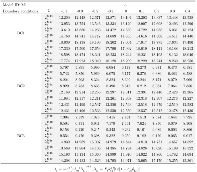
In this section, vibration of circular and parabolic cylindrical panels having variable thicknesses along their circumferences or axes is studied. Three sets of the models with circular profile and also three more sets of the models with parabolic profile are constructed. Besides, each set has two sub-sets of the models with variable thicknesses. One subset is corresponding to the models having vari-able thicknesses along their circumferences (represented by MNs), while the other subset is includ-ing the models with variable thicknesses along their axes (represented by MNx). For each of the subsets, three cases for the boundary conditions are considered. General characteristics for all inves-tigated models are introduced in Table 8. Variation of frequency parameter against thickness pa-rameter α is presented in Tables 9-11 for the case of circular models. Frequency parameter for the models having a variable thickness along their axis varies in a manner completely reverse to that of the models having variable thickness along their circumference for the BC1 boundary conditions.
(
)
(
)
2 3
0 11 11 1 0 21 12
0.5
, [12 1 ]
i ia h D D E h
l =w r = -J J
Table 9: Variation of natural frequency parameter for M1x and M1s models.
a
Model ID: M1
Latin American Journal of Solids and Structures 12 (2014) 2099-2121
In addition, it is observed that variation of first frequency parameter against the thickness parame-ter is linear upwards or downwards for both of the models having variable thickness along their axis or circumference for the BC1 boundary conditions.
( )
3
2 0 1 0
11
11 21 12
, 12 1 i i E h h a D D r l w J J = =
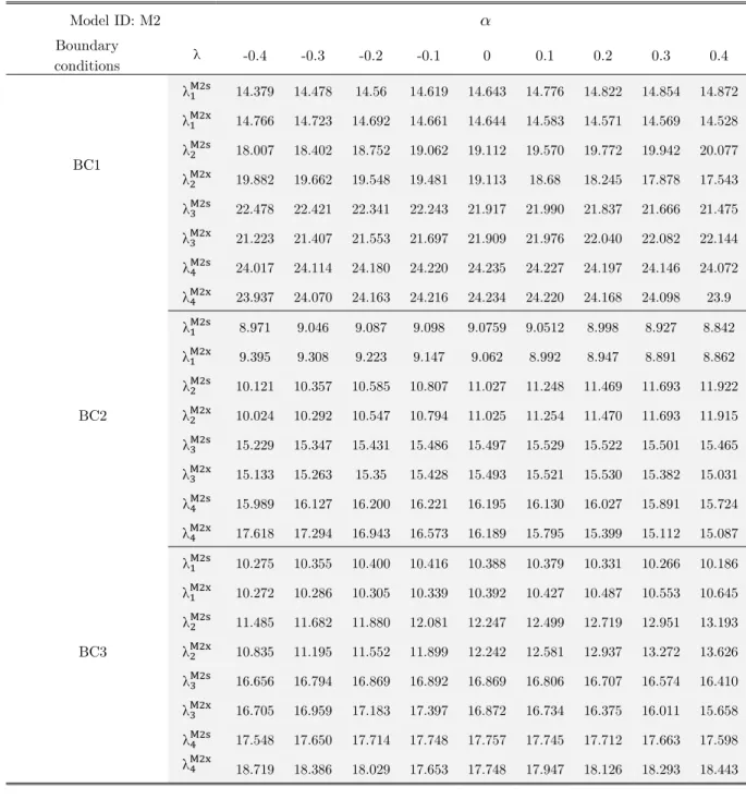
-Table 10: Variation of natural frequency parameter for M2x and M2s models
a
Model ID: M2
Latin American Journal of Solids and Structures 11 (2014) 2099-2121 Tables 9 to 11 show the variation of frequency parameter against thickness parameter for circular cylindrical shells, when their boundary conditions are of BC2 or BC3 types. In comparison with the results explained for the case of the BC1 boundary condition, the frequency parameter varies at the same manner against thickness parameter for the models having variable thickness along their axis and the models having variable thickness along their circumference, when the boundary conditions are of either BC2 or BC3 types.
From the results summarized in Tables 9 to 11, it is observed that with increase in the value of C/b for the models, frequency parameter is also increased.
a
Model ID: M3
0.4 0.3 0.2 0.1 0 -0.1 -0.2 -0.3 -0.4 λ Boundary Conditions 16.421 16.504 16.578 16.644 16.701 16.752 16.799 16.840 16.878 λ BC1 17.217 17.084 16.952 16.823 16.696 16.572 16.448 16.324 16.195 λ 20.077 19.981 19.850 19.684 19.543 19.246 18.972 18.658 18.305 λ 18.440 18.789 19.146 19.507 19.565 20.219 20.583 20.890 21.196 λ 25.219 25.520 25.787 25.855 25.908 25.916 25.909 25.876 25.817 λ 25.930 25.976 25.999 25.998 25.939 25.909 25.816 25.608 25.337 λ 25.57 25.692 25.799 26.056 26.242 26.506 26.694 26.855 26.981 λ 26.644 26.577 26.483 26.364 26.248 26.044 25.843 25.683 25.506 λ 10.013 10.078 10.129 10.166 10.187 10.188 10.167 10.120 10.042 λ 10.193 10.177 10.173 10.177 10.190 10.210 10.233 10.258 10.283 λ 15.118 15.204 15.217 15.145 14.996 14.790 14.547 14.277 13.985 λ 14.525 14.806 15.047 15.181 15.129 14.917 14.619 14.271 13.883 λ BC2 16.822 16.593 16.411 16.282 16.195 16.124 16.042 15.927 15.761 λ 17.017 16.741 16.512 16.391 16.182 16.663 16.942 17.248 17.555 λ 19.251 19.276 19.280 19.265 19.230 19.166 19.076 18.952 18.787 λ 19.292 19.311 19.308 19.283 19.233 19.154 19.043 18.893 18.696 λ 11.815 11.877 11.924 11.954 11.966 11.956 11.923 11.862 11.767 λ 12.690 12.490 12.304 12.132 11.970 11.818 11.674 11.535 11.471 λ 16.047 16.152 16.211 16.217 16.162 16.047 15.882 15.679 15.450 λ 15.578 15.905 16.154 16.343 16.260 16.121 15.727 15.266 14.762 λ BC3 18.308 18.015 17.749 17.515 17.475 17.143 16.982 16.810 16.603 λ 18.934 18.475 18.047 17.688 17.503 17.569 17.777 18.030 18.291 λ 21.214 21.276 21.315 21.331 21.321 21.285 21.216 21.111 20.960 λ 22.316 22.089 21.849 21.595 21.324 21.034 20.721 20.383 20.012 λ ( ) 3
2 0 1 0
11
11 21 12
, 12 1 i i E h h a D D r l w J J = =
Latin American Journal of Solids and Structures 12 (2014) 2099-2121
In Tables 12 to 14, variation of frequency parameter against thickness parameter (α), for parabolic models is presented. Similar to the results for circular models, it is observed herein also that with any increase in the value of C/b for the models with parabolic profile, frequency parameter increas-es. The tendencies of the variation of frequency parameter for the models having parabolic profile are the same as those for the models having circular profile. Nevertheless, frequency parameter for the parabolic models is greater than that for the circular models, as confirmed also in Cheung and Cheung (1972).
a
Model ID: M4
0.4 0.3 0.2 0.1 0 -0.1 -0.2 -0.3 -0.4 λ Boundary Conditions 13.648 13.556 13.471 13.308 13.151 12.973 12.771 12.545 12.295 λ BC1 12.416 12.620 12.649 13.044 13.181 13.480 13.696 13.908 14.111 λ 15.250 15.011 14.946 14.884 14.836 14.356 14.114 13.960 13.787 λ 14.680 14.746 14.723 14.843 14.878 14.908 14.933 14.955 14.974 λ 17.683 17.816 17.923 18.089 18.227 18.315 18.274 18.206 18.108 λ 18.353 18.382 18.363 18.289 18.211 18.059 17.921 17.767 17.596 λ 18.141 18.224 18.256 18.318 18.339 18.364 18.498 18.626 18.744 λ 18.525 18.462 18.403 18.377 18.342 18.288 18.195 18.080 17.931 λ 6.7155 6.606 6.486 6.405 6.309 6.215 6.120 6.026 5.927 λ 6.720 6.615 6.451 6.409 6.308 6.205 6.099 5.990 5.8735 λ 8.081 8.191 8.245 8.356 8.418 8.436 8.437 8.405 8.336 λ 7.966 8.076 8.142 8.324 8.441 8.602 8.748 8.896 9.043 λ BC2 12.459 12.511 12.526 12.529 12.477 12.432 12.387 12.343 12.297 λ 12.365 12.414 12.420 12.456 12.445 12.411 12.349 12.255 12.121 λ 12.729 12.653 12.646 12.611 12.636 12.643 12.630 12.592 12.523 λ 12.528 12.570 12.591 12.630 12.644 12.644 12.627 12.590 12.526 λ 7.859 7.777 7.685 7.645 7.592 7.545 7.504 7.467 7.432 λ 8.440 8.209 7.871 7.756 7.592 7.309 7.086 6.861 6.633 λ 9.005 9.109 9.184 9.270 9.321 9.350 9.355 9.328 9.266 λ 9.122 9.170 9.229 9.290 9.359 9.432 9.508 9.587 9.666 λ BC3 14.736 14.798 14.885 14.944 15.025 15.095 15.102 15.084 15.033 λ 15.413 15.335 15.269 15.061 14.999 14.520 14.271 14.000 13.705 λ 14.790 14.879 14.913 15.021 15.065 15.105 15.183 15.254 15.310 λ 15.498 15.347 15.312 15.160 15.036 14.890 14.722 14.528 14.305 λ ( ) 3
2 0 1 0
11
11 21 12
, 12 1 i i E h h a D D r l w J J = =
Latin American Journal of Solids and Structures 11 (2014) 2099-2121 α Model ID:M5 0.4 0.3 0.2 0.1 0 -0.1 -0.2 -0.3 -0.4 λ Boundary Conditions 15.465 15.438 15.414 15.322 15.254 15.169 15.063 14.956 14.838 λ BC1 15.115 15.123 15.153 15.187 15.234 15.286 15.348 15.413 15.471 λ 21.463 21.272 21.047 20.641 20.066 20.042 19.966 19.795 19.295 λ 18.383 18.822 19.325 19.668 20.062 20.443 20.798 21.014 20.839 λ 21.939 22.17 22.311 22.389 22.494 22.586 22.652 22.728 22.732 λ 21.736 21.673 21.593 21.515 20.962 20.615 20.169 20.123 20.416 λ 25.456 25.534 25.549 25.583 25.571 25.535 25.477 25.381 25.254 λ 25.227 25.366 25.470 25.541 25.577 25.575 25.535 25.451 25.320 λ 9.4718 9.556 9.575 9.680 9.714 9.726 9.714 9.6724 9.595 λ 9.466 9.513 9.5134 9.639 9.7235 9.794 9.882 9.985 10.071 λ 12.758 12.533 12.237 12.086 11.864 11.641 11.415 11.183 10.942 λ 12.745 12.527 12.419 12.073 11.841 11.617 11.362 11.118 10.846 λ BC2 15.900 15.931 15.943 15.950 15.934 15.900 15.842 15.756 15.635 λ 15.772 15.937 15.945 15.948 15.920 15.884 15.822 15.739 15.616 λ 16.436 16.593 16.633 16.818 16.880 16.902 16.880 16.805 16.668 λ 15.471 15.672 16.081 16.487 16.887 17.275 17.648 17.999 18.323 λ 10.778 10.858 10.902 10.970 10.999 11.007 10.992 10.944 10.864 λ 11.197 11.123 11.075 11.022 10.991 10.965 10.954 10.946 10.941 λ 14.041 13.798 13.593 13.340 13.123 12.912 12.706 12.502 12.297 λ 14.574 14.155 13.831 13.450 13.119 12.761 12.406 12.052 11.687 λ BC3 17.339 17.255 17.397 17.481 17.543 17.565 17.543 17.471 17.336 λ 16.376 16.754 17.059 17.269 17.543 17.971 17.754 17.523 17.288 λ 18.053 18.111 18.136 18.181 18.188 18.175 18.137 18.070 17.966 λ 18.758 18.614 18.454 18.280 18.197 18.246 18.629 18.992 19.295 λ ( ) 3
2 0 1 0
11
11 21 12
, 12 1 i i E h h a D D r l w J J = =
Latin American Journal of Solids and Structures 12 (2014) 2099-2121 a Model: M6 0.4 0.3 0.2 0.1 0 -0.1 -0.2 -0.3 -0.4
λ
Boundary conditions 16.994 17.011 17.022 17.026 17.023 17.103 17.202 17.532 17.763 λ B.c1 17.501 17.321 17.251 17.140 17.037 16.941 16.850 16.761 16.670 λ 21.921 21.840 21.721 21.563 21.364 21.126 20.846 20.505 20.153 λ 20.150 20.577 20.998 21.126 21.350 22.265 22.666 23.046 23.397 λ 25.505 25.748 25.966 26.167 26.346 26.507 26.646 26.762 26.854 λ 26.914 26.806 26.675 26.528 26.360 26.170 25.956 25.715 25.442 λ 27.328 27.440 27.511 27.562 27.575 27.555 27.502 27.415 27.292 λ 27.564 27.668 27.730 27.772 27.783 27.759 27.696 27.588 27.429 λ 10.605 10.668 10.718 10.752 10.770 10.768 10.745 10.694 10.611 λ 10.717 10.717 10.727 10.746 10.774 10.808 10.846 10.887 10.929 λ 15.962 16.129 16.263 16.361 16.511 16.364 16.136 15.823 15.480 λ 15.464 15.803 16.145 16.479 16.553 16.397 16.035 15.644 15.225 λ B.c2 18.177 17.845 17.521 17.203 16.960 16.652 16.536 16.447 16.315 λ 18.185 17.852 17.519 17.195 17.019 17.274 17.608 17.945 18.269 λ 19.221 19.223 19.208 19.174 19.119 19.041 18.937 18.799 18.622 λ 19.162 19.182 19.183 19.164 19.122 19.054 18.956 18.822 18.644 λ 12.296 12.355 12.399 12.426 12.435 12.424 12.389 12.325 12.229 λ 13.052 12.879 12.721 12.574 12.439 12.313 12.195 12.084 11.974 λ 16.899 17.052 17.172 17.256 17.394 17.270 17.157 16.942 16.651 λ 16.417 16.725 17.039 17.347 17.444 17.353 17.146 16.645 16.111 λ B.c3 19.611 19.246 18.897 18.567 18.283 17.977 17.749 17.577 17.419 λ 20.200 19.705 19.218 18.743 18.309 18.177 18.417 18.706 18.991 λ 21.250 21.281 21.292 21.281 21.248 21.189 21.099 20.975 20.807 λ 22.163 21.957 21.736 21.501 21.248 20.977 20.683 20.364 20.013 λ ( ) 32 0 1 0
11
11 21 12
, 12 1 i i E h h a D D r l w J J = =
Latin American Journal of Solids and Structures 11 (2014) 2099-2121 From the obtained numerical results, the following observations can be summarized:
With increase in C/b (b is constant and C varies), frequency of all models (circular and parabolic profiles) is increased. With increase in C/b, arc length of both profiles will increase, and then weight of models increases. In addition, the increase of camber (C) will decrease radius of curva-ture of shells. Increase in the weight of the models decreases the natural frequency and also de-crease of the radius of curvature inde-creases the natural frequency of models. Therefore, effect of the change in the curvature on the natural frequency is greater than the effect of change in the weight for studied models. The tendencies of variation of frequency parameter are the same for both cir-cular and parabolic models. Nevertheless, for the models with the same values of C/b, the natural frequency in case of parabolic curvature is greater than that in case of circular curvature. This phenomenon may be due to the facts that; (1) local stiffness of parabolic models is greater than local stiffness of circular models and (2) weight of circular models is greater than parabolic models with the same C/b (because the arc length of circular profile is greater than the arc length of par-abolic profile).
Effect of thickness variation along both directions on the natural frequency is studied. It was aimed to find out the difference between effect of thickness variation along direction with zero curvature (x direction) and effect of thickness variation along direction with nonzero curvature (s direction). It is observed that for the case of BC1 boundary condition, the frequency parameter variation for the models with variable thickness along their axis is in opposite tendency compared with the models having variable thickness along their circumference.
Effect of boundary condition on natural frequency is studied for three cases. It can be seen that the effect of boundary condition on natural frequency is greater than the effect of variable thick-ness on natural frequency. Models with BC1 boundary condition have largest natural frequency and models with BC2 boundary condition have lowest natural frequency. In addition, boundary condition changes the manner of frequency parameter variation against the thickness parameter. For example, for the BC1 type of boundary condition, frequency parameter varies linearly against thickness parameter but for the BC2 and BC3 types of boundary condition, frequency parameter varies nonlinearly against thickness parameter.
3.3 Effect of variable thickness on the mode shapes
Latin American Journal of Solids and Structures 12 (2014) 2099-2121
model (the parabolic cylindrical shell with variable thickness along s axis). As can be observed, the thickness parameter does not have any significant effect on the mode shape for M5s model.
Mode number
1st 2nd 3rd 4th
-0.
4
-0.
2
0
0.
2
0.
4
Figure 3: Effect of thickness parameter ( ) on the mode shapes for the parabolic model with
Latin American Journal of Solids and Structures 11 (2014) 2099-2121
Figure 4: Effect of thickness parameter ( ) on the mode shapes for the parabolic model with . 5 (Model M6x).
Mode number
1st 2nd 3rd 4th-0.4
-0.2
0
0.2
Latin American Journal of Solids and Structures 12 (2014) 2099-2121 4 CONCLUSIONS
An approximate analysis method for investigating the free vibration behavior of circular and para-bolic cylindrical shells having variable thickness along their axis or circumference is presented. A finite element method based on B-spline functions is further extended to find out the natural fre-quencies and corresponding mode shapes for the cylindrical shells with variable radii of curvature and non-uniform thicknesses. Usefulness and accuracy of the present method is demonstrated through comparison of the results for a variety of cases. It is observed that frequency parameter for circular models vary in the same way against thickness parameter as that for parabolic models. Moreover, natural frequency of cylindrical models with a parabolic profile is slightly greater than that of cylindrical models with a circular profile.
References
Ashour, A.S., (2001). A semi-analytical solution of the flexural vibration of orthotropic plates of variable thickness, Journal of Sound and Vibration 240: 431–445.
Cheng, S.P., Chuang, D., (1990). Dynamic analysis of stiffened plates and shells using spline gauss collocation meth-od, Computers & Structures 36: 623-629.
Cheng, S.P., Dade, H., Zongmu, W., (1987). Static, vibration and stability analysis of stiffened plates using B spline functions, Computers & Structures27:73-78.
Cheung, Y. K., Cheung, M.S., (1972). Vibration analysis of cylindrical panels, Journal of Sound and Vibration 22: 59-73.
Duan, W., Koh, C., (2008). Axisymmetric transverse vibrations of circular cylindrical shells with variable thickness, Journal of Sound and Vibration 317: 1035–1041.
Grigorenko, A.Y., Parkhomenko, A.Y., (2011). Free Vibration of Shallow Orthotropic Shells with Variable Thickness and Rectangular platform, Journal of International Applied Mechanics 46: 877-889.
Grigorenko, Y.M., Grigorenko, A.Y., Efimova, T.L., (2008). Spline-based investigation of natural vibrations of ortho-tropic rectangular plates of variable thickness within classical and refined theories, Journal of Mechanics of Materials and Structures 3: 929-952.
Huang, M., Ma, X.Q., Sakiyama, T., Matsuda, H., Morita, C., (2005). Free vibration analysis of orthotropic rectan-gular plates with variable thickness and general boundary conditions, Journal of Sound and Vibration 288: 931-955. Huang, M., Ma, X.Q., Sakiyama, T., Matsuda, H., Morita, C., (2007). Free vibration analysis of rectangular plates with variable thickness and point supports, Journal of Sound and Vibration 300: 435-452.
Khalifa, A.M., (2011). Simplified equations and solutions for the free vibration of an orthotropic oval cylindrical shell with variable thickness, Math. Meth. Appl. Sci 34: 1789-1800.
Pellicano, F., (2007). Vibrations of circular cylindrical shells: theory and experiments, Journal of Sound and Vibra-tion 303: 154–170.
Sakiyama, T., Huang, M., (1998). Free vibration analysis of rectangular plates with variable thickness, Journal of Sound and Vibration 216: 379–397.
Sivadas, K., Ganesan, N., (1991). Free vibration of circular cylindrical shells with axially varying thickness, Journal of Sound and Vibration 147: 73–85.
Latin American Journal of Solids and Structures 11 (2014) 2099-2121 Srinivasan, R.S., Bobby, W., (1976). Free vibration of noncircular cylindrical shell panels, Journal of Sound and Vibration 46: 43-49.
Suzuki, K., Leissa, A., (1985).Free vibrations of noncircular cylindrical shells having circumferentially varying thick-ness, Journal of Applied Mechanics52: 149–154.
Yamada, G., Irie, T., Notoya, S., (1999). Natural frequencies of elliptical cylindrical shells, Journal of Sound and Vibration 101: 133–139.
Zhang, L., Xiang, Y., (2006). Exact solutions for vibration of stepped circular cylindrical shells, Journal of Sound and Vibration 299: 948–964.