Abstract
The estimation of the value and direction of post-liquefaction defor-mations is one of the most challenging issues in the modelling of liquefaction soil, due to the inherent and induced anisotropy. It is very important in the science of soil-constitutive models to present a simple and comprehensive model for the prediction of fabric anisot-ropy effects in pre- and post-liquefaction behaviour in granular soil. In the framework of the multilaminate method, 17 planes with pre-determined directions are defined, instead of defining all occurrences depending on the direction in three planes perpendicular to each other in a Cartesian coordinate system. As a result, calculation ac-curacy is increased in the point due to the effectiveness of the behav-iours in different directions. In the present study, after modifying an advanced model by removing constants related to the fabric effect and using lower constants, the precision of model performance after the removal of constants was studied and compared with experi-mental results in different monotonic, cyclic, drained, and undrained loading conditions. After this, the formation of stress and strain in 17 planes was evaluated in terms of pre- and post-liquefaction, with monotonic and cyclic loadings. The study of the curves shows in-duced anisotropy in different directions of sandy soil and thus proves the capability of the model in this regard.
Keywords
multi-directional, granular materials, anisotropy, undrained, lique-faction, cyclic.
Modification of a Constitutive Model in the Framework
of a Multilaminate Method for Post-Liquefaction Sand
1 INTRODUCTION
Saturation soil without cohesion undergoes flow failure with huge displacements during rapid static loading or earthquakes. Therefore, it is very important to study the post-liquefaction conditions of sandy soil, due to their significant effects on related structures. Some researchers have evaluated
post-Hadi Dashti a, *
Seyed Amirodin Sadrnejad b Navid Ganjian a
a Department of Civil Engineering, Science
and Research Branch, Islamic Azad University, Tehran, Iran.
b Dept. of Civil Eng, K.N. Toosi
University of Tech., Tehran, Iran
* Corresponding author:
E-mail: hdashti1356@yahoo.com
http://dx.doi.org/10.1590/1679-78253841
liquefaction displacements by using a set of experimental and centrifuge tests in different conditions (Ishikawa et al., 2015; Wang et al., 2015; Basari and Ozden, 2013). Wang et al. (2015) studied post-liquefaction soil in cyclic loading under different post-post-liquefaction reconsolidations. Their study was conducted on silt soil. It has been observed that if post-liquefaction soil has undergone monotonic loading, soil shear strength and stiffness is increases due to increasing post-liquefaction reconsolidation percent. In addition, it has been observed that the critical state line is different in pre- and post-liquefaction stages. Ishikawa et al. (2015) studied post-post-liquefaction progressive failure of shallow foun-dations in centrifuge tests. An important point in induced deformation resulting from liquefaction is its slow movement (several minutes) compared to the shaking duration of an earthquake (several tens of milliseconds). They proved that post-liquefaction progressive failure in shallow foundations results from the spread of the local shear boundaries of the liquefaction layer. Settlement and tilting occur in complete liquefaction, even after the earthquake. Shamoto et al. (1998) divided deformations re-sulting from liquefaction into two categories: volumetric deformations (which caused settlement) and shear deformations (which caused lateral spreading). They presented a method to simultaneously predict these two displacements in terms of their effect on each other.
A few researchers have studied issues related to post-liquefaction conditions of sand particles using numerical models (Elgmal et al., 2002; Zang and Wang, 2012; Sadrnejad, 2007). Elgmal et al. (2002) introduced a constitutive model to predict liquefaction and numerically studied the effect of the fre-quency content of input excitation on the post-liquefaction shear deformation. They proved that dominant excitation frequency had the most significant effect on post-liquefaction soil response. Low excitation frequency creates many lateral deformations. Post-liquefaction shear deformation is one of the challenging subjects in liquefaction soil modelling. Zang and Wang (2012) presented a numerical algorithm and its application in a theoretical framework to predict post-liquefaction deformations of saturation sand under cyclic and undrained loadings. They considered the post-liquefaction mecha-nism by decomposition of volumetric strain into three components with a certain physical background. The interaction between these components controls the post-liquefaction deformations and determines changes in these three physical states in the liquefaction process. This assumption determines the complex issue of transfer of small pre-liquefaction displacements to large post-liquefaction displace-ments.
Sand particles are formed under different environmental conditions during their lifetime. Bedding plane gradient leads to the formation of weak and strong planes in different directions. The initial anisotropy causes different behaviour of sand in different loading conditions. Another type of anisot-ropy seen in granular materials is under loading effect and the production of plastic strain in different directions. This type of anisotropy is known as induced anisotropy. There are important effects on the behaviour of sandy soil in different conditions. The three important features of granular soil are liquefaction, dilation, and critical state that can be produced during one loading; these are all affected by induced anisotropy. The post-liquefaction behaviour of sand particles and the direction of their deformations are affected by initial and induced anisotropy, due to the effect of initial anisotropy and the history of stress and strain.
between microscopic and macroscopic structures (Guo and Zhao,2013;Yang et al., 2008; Yang et al., 2013; Hicher and Chang, 2007; Kruyt and Rothenburg, 2016; Khalili and Mahboubi, 2014;Voiadjis et al., 1995; Kruyt and Rothenburg, 2014; Guo, 2014; Li and Yu, 2014; Yan, 2009; Chang and Hicher, 2005). Other studies have been conducted to predict the fabric anisotropic behaviour using different parameters and placing them in equations of constitutive model of soil (Yu et al., 2013; Yang et al., 2008; Gao et al., 2014; Dafalias and Manzari, 2004; Lashkari, 2009; Zhao and Guo, 2013; Dafalias et al., 2004). In addition, a few studies have been conducted to consider the effect of induced anisotropy by using constitutive models (Hareb and Doanh, 2012; Tang Tron Tran et al., 2014; Ye et al., 2012). Although various models have been presented to predict sandy soil behaviour in different loading conditions (Zang and Wang, 2012; Yang et al., 2008; Dafalias and Manzari, 2004; Lashkari, 2009; Liu et al., 2016; Wang and Xie, 2014; Li, 2002; Wang et al., 2014), such models either have been used in restrictive anisotropic conditions and limited loading conditions or they have used a high number of material constants. Most models are not able to determine the parameters dependent on direction, such as fabric, by using stress and strain invariants. Therefore, the multilaminate constitutive model— also known as micro-plane in some sources (Bazant et al., 1996; Caner and Bazant, 2000)—is a suitable mechanism for the simultaneous prediction of complete anisotropy in sandy soil in terms of material behaviour in different planes. This model has been evaluated for different materials, such as soil (Sadrnejad et al., 2009; Sadrnejad, 2009; Sadrnejad and Karimpour, 2011), and for the estimation of damage models in concrete (Ghadrdan and Sadrnejad, 2015; Sadrnejad and Labibzadeh, 2006). Some researchers considered 13 planes in different directions of a sphere with a radius of one; they modelled effects of anisotropy for different models (Sadrnejad, 2009; Sadrnejad and Karimpour, 2011; Sadrnejad and Labibzadeh, 2006). The recent model has been problematic due to the number of planes, preparation of simultaneous conditions, strain consistency, and equilibrium (Ghadrdan and Sadrnejad, 2015; Sadrnejad and Labibzadeh, 2006).
2 MULTILAMINATE MODEL
The multilaminate theory (Sadrnejad, 2011) is based on the determination of numerical relationship between micro-scale behaviours and engineering mechanical properties (macro scale behaviour) in form of constitutive equation. In other words, material properties are obtained by features of each constitutive element and stress-strain behaviour of material is obtained by studying micro scale be-haviour.
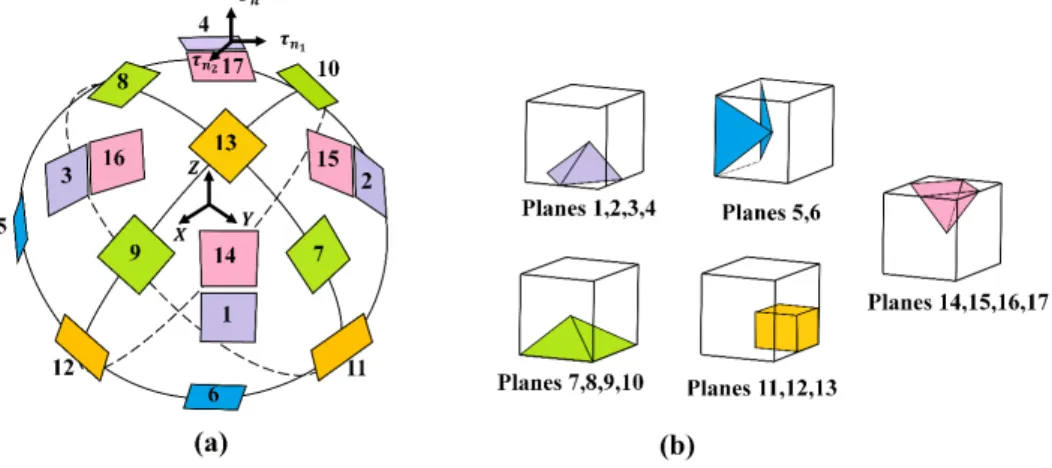
When a multi-dimensional part undergoes small shear stress, it carries elastic shear deformation. Multi-dimensional parts start moving in the direction of boundary planes—known as sliding planes— due to the increase in stress and reaching to a certain amount of stress. Shear stress that creates higher deformation is increased by increasing deformation. The total shear deformation is the sum of elastic shear deformation in multi-dimensional parts and plastic shear deformation resulting from the sliding of adjacent parts. When stress is decreased, the elasticity component returns to the starting point. Then, the multi-dimensional parts start sliding inversely due to the reduction in stress, and reaches a certain value. The shear stress required for sliding depends on the normal stress. Sliding occurs when the stress state crosses the yield limit. However, sliding occurs only in sliding planes in the suggested directions (schematic view in Figure 1). On the basis of this, the higher the number of pre-determined planes, the closer to the reality will be the sliding, opening, and closing of the planes. In the multilaminate theory, the numerical integral from a mathematical function is determined by spreading in a sphere area with radius of one. Such a mathematical function can express the changes in the physical properties of a sphere area. For determining the numerical integral, the hy-pothetical sphere area with a radius of one can be approximated with several flat planes tangential to different points of the sphere area (Figure 2(a)). Each plane has a contact point with the sphere surface; thus, by limiting such planes, the number of contact points or basic points can be defined. When calculating numerical integral, the quantity spread on sphere surface area can be obtained in the mentioned points. The numerical integral is obtained from the continuous function off x y z( , , )on the sphere surface (the sum of the values off x y z( , , )in sample points that is multiplied by the weight coefficients related to the points). The number of sample points should be increased in order to reduce errors. The following relation shows the relationship between the numerical integral and the normal integral:
W =
å
=òò
( )1
( , , ) 4 ( , , )
n
i i i i
i
f x y z dxdydz p w f x y z (1)
Ω = sphere area n = number of points
w(i) = weight coefficient of point i fi(xi,yi,zi) = value of function f in point i
Figure 1: (a) Presentation of real accumulation of particles (b) 2D presentation of accumulation of artificial multi-dimensional parts.
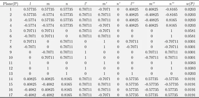
To display the geometry of planes properly, in the present model, the tangential planes for such micro-planes are shown in hemispheres with a radius of one, as shown in Figure 2(a). Figure 2(b) shows their locations inside the unit cubic, while Table 1 indicates the directional cosines, the shear stress directions tn1 and tn2 , and the weight coefficients of 17 planes.
Figure 2: The position of 17 planes a) on the sphere surface b) inside the cubic.
If l, m, and n are directional cosines perpendicular to the plane, l¢,m¢, and n¢ are directional cosines for shear stress direction
1 n
t , and l¢¢, m¢¢, and n¢¢ are directional cosines of shear stress
direction 2 n
t . According to the results of Sadrnejad and Labibzadeh (2006), stress values in planes
can be obtained by the following relation, using matrix algebraic relations and regarding the amount of stress at the point :
1
2
( )
n xx xy xz
P n yx yy yz
zx zy zz n
l m n l
l m n m
l m n n
s s t t
t t s t
t t s
t
é ù é ù é ù é ù
ê ú ê ú ê ú ê ú
ê ú ê ¢ ¢ ¢ú ê ú ê ú =ê ú =ê ú ê ú ê ú ê ú ê ¢¢ ¢¢ ¢¢ú ê ú ê ú ê ú êë ú êû ë ú ê úû ë û ë û
σ (2)
Here, sn is stress perpendicular to the plane, and tn1 and tn2 are shear stresses in planes in
yz
t , tyx, tzx, and tzy are shear stresses at the point. In the present research, given the lack of body
forces, we have txy = tyx, txz = tzx, and tyz = tzy.
Plane(P) l m n l' m' n' l'' m'' n'' w(P)
1 0.57735 0.57735 0.57735 0.70711 -0.7071 0 0.40825 0.40825 -0.8165 0.0203
2 0.57735 -0.5774 0.57735 0.70711 0.70711 0 0.40825 -0.40825 -0.8165 0.0203
3 -0.5774 0.57735 0.57735 0.70711 0.70711 0 0.40825 -0.40825 0.8165 0.0203
4 -0.5774 -0.5774 0.57735 0.70711 -0.7071 0 0.40825 0.40825 0.8165 0.0203
5 0.70711 0.70711 0 0.70711 -0.7071 0 0 0 1 0.0581
6 -0.7071 0.70711 0 0.70711 0.70711 0 0 0 1 0.0581
7 0.70711 0 0.70711 0 1 0 0.70711 0 -0.70711 0.0301
8 -0.7071 0 0.70711 0 1 0 -0.7071 0 -0.70711 0.0301
9 0 -0.7071 0.70711 1 0 0 0 0.70711 0.70711 0.0301
10 0 0.70711 0.70711 1 0 0 0 -0.70711 0.70711 0.0301
11 1 0 0 0 1 0 0 0 1 0.0383
12 0 1 0 1 0 0 0 0 1 0.0383
13 0 0 1 0 1 0 1 0 0 0.0203
14 0.40825 0.40825 0.8165 0.70711 -0.7071 0 0.57735 0.57735 -0.57735 0.0191
15 0.40825 -0.4082 0.8165 0.70711 0.70711 0 0.57735 -0.57735 -0.57735 0.0191
16 -0.4082 0.40825 0.8165 0.70711 0.70711 0 0.57735 -0.57735 0.57735 0.0191
17 -0.4082 -0.4082 0.8165 0.70711 -0.7071 0 0.57735 0.57735 0.57735 0.0191
Table 1: Directional cosines and weight coefficients of 17 planes.
After the calculation of stress within planes by the use of transfer relation, elastic and plastic strains are calculated in the planes by the use of relations of the constitutive model. As a result, the strains calculated in planes are transferred to the point by the following relation. The relation is equivalent to the relation of stress transfer from planes to points, as presented by Sadrnejad and Labibzadeh (2006):
17
( ) ( ) ( ) 1
6
ij P P P
P
w
e
=
é ù é ù
= ´
å
êëT ú êû ëε úû (3)( )P
ε is strain that is equivalent to stresses in planes and w( )P is the weight coefficient of planes and
ij
e is the six-component strain in point:
xx
yy
zz ij
xy
yz
xz
e e e e
g g g
ì ü
ï ï
ï ï
ï ï
ï ï
ï ï
ï ï
ï ï
ï ï
ï ï
= íï ýï
ï ï
ï ï
ï ï
ï ï
ï ï
ï ï
ï ï
ï ï
î þ
(4)
( )P
T is plane transfer matrix. The value of ( )P
2
2
2
( )
1 / 2( ) 1 / 2( ) 1 / 2( ) 1 / 2( ) ln 1 / 2( ) 1 / 2( ) P
l ll l l
m m m m m
n n n n n
lm l m m l m l l m
mn m n n m m n n m
l n n l l n n l
é ¢ ¢¢ ù
ê ú
ê ¢ ¢¢ ú
ê ú
ê ¢ ¢¢ ú
ê ú
= ê ú
ê ¢ + ¢ ¢¢ + ¢¢ ú
ê ú
ê ¢ + ¢ ¢¢ + ¢¢ ú
ê ú
ê ¢ + ¢ ¢¢ + ¢¢ ú
ê ú
ë û
T (5)
3 CONSTITUTIVE MODEL IN THE PLANE
Among the different models representing sand behaviour in liquefaction soil, the model given by Dafalias and Manzari (2004) has remarkable features. Consistent with the principles of limited soil mechanic, definition of bounding surface, and dilatancy surface, and their dependency on state pa-rameter y , and them change during loading and eventually their match with critical surface in failure condition, cause correct prediction of dilation and contraction of dense and loose sand particles (com-pared to critical state line) and their softening. In the present research, according to the multilaminate framework for the prediction of fabric anisotropy effects, parameters related to the fabric effect of sandy soil particles were omitted from the equation, while low constants were used in different con-ditions compared to the initial model. According to these features, for the better performance of the mentioned model and to use it in different loading conditions and increase efficiency, the model given by Dafalias and Manzari (2004) was used as the constitutive model in 17 planes via the multilaminate method. In the following section, governing equations to planes and modifications were dealt with using the equations given by Dafalias and Manzari (2004). It should be noted that in all equations, the index ‘
P
’ in parentheses means the number of the planes and bold expressions show tensor variables.3.1 Elastic Constitutive Model in the Plane
In the framework of hypo-elastic theory, the elastic shear modulus G( )P and the elastic bulk modulus
( )P
K , as functions of void ratio e and stress perpendicular to the plane sn P( ), are defined as follows:
= - 2 + ( ) 1/2
( ) 0 (2.97 ) / (1 )( )
n P
P P atm
atm
G G P e e
P
s
(6)
and
( ) ( )
2(1 )
3(1 2 )
P
P P
P
K n G
n + =
- (7)
3.2 Critical State Line
In this model, the soil limit state theory is used in planes. According to this theory, the critical void ratio
e
c(P) and the normal stress sn P( ) are exponentially inter-related in planes via the followingrelation:
= - ( )
( ) 0 ( )P
n P
c P P cP
atm
e e
P x
s
l (8)
0P
e and lcP are the model constants in the plane. The state parameter y( )P is defined as follows for
each plane:
( )P e( )P ec P( )
y = - (9)
( )P
e is equal to e at the beginning of the loading. Bounding, dilatancy, and critical surfaces are defined
using this parameter. Depending on the change in this parameter during loading, the aforementioned surfaces were variable as well, leading to the prediction of some features of sand, such as phase change of dilation, softening, and compatibility with limit state theory.
3.3 Yield Surface
Yield surface function in the plane is defined by the following equation:
1/2
( )P [( ( )P n P( ) ( )P ) : ( ( )P n P( ) ( )P )] 2 / 3 n P( ) P 0
f = S -s α S -s α - s m = (10)
( )P
α is the deviatoric back stress ratio tensor. This component is used to determine the yield surface axis. The sign ‘:’ means the trace and multiplication of two tensors. Equation f( )P is cone geometry
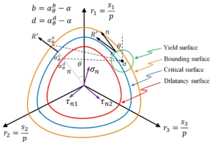
in the deviatoric stress space of the plane. Figure 3 indicates the schematic of yield, dilatancy, bound-ing, and critical surfaces at the point, and they are observed similarly in the plane. mP is one of the plane's constants and the deviatoric stress tensor S( )P in the plane, is calculated as follows:
( )P = ( )P -sn P( ) ( )P
S σ I (11)
where:
( )
1 0 0 0 0 0 0 0 0
P
é ù
ê ú
ê ú
= ê ú
ê ú
ê ú
ë û
I (12)
( )P
r is stress ratio tensor in the plane. It is calculated by following equation:
( )P = ( )P /sn P( )
Figure 3: Schematic of yield surface, dilatancy surface, bounding surface, and critical
surface at the point and in axes space σn,
1 n
t and
2 n
t in the plane.
According to equation of f( )P , the yield surface gradient in space r( )P is obtained as follows:
( )P = ¶f( )P /¶ ( )P
L σ (14)
( )P
n , i.e. the tensor perpendicular to the yield surface in the deviatoric stress space in the plane, is
defined as follows:
( ) ( ) ( )
( ) ( )
P P
P
P P
-=
-r α
n
r α (15)
where shows tensor norm.
3.4 Changes in Plastic Strain
Plastic strain increment is calculated from the following relation:
=
( ) ( ) ( )
P
P P P
dε L R (16)
Here, L( )P is the loading index or plastic coefficient, are Macaulay’s brackets, and x is
equal to x if x >0, while it is equal to zero if x £0.R( )P is the vector direction ( ) P
P
dε . In this
model and in general, R( )P ¹ ¶f( )P /¶σ( )P , meaning that the non-associated flow rule is governed in
plasticity. R( )P is divided into two deviatoric and volumetric parts using the following relation. The
2
( ) ( ) ( ) ( ) ( ) ( ) ( ) ( ) ( ) ( ) ( )
1 1 1
( )
3 3 3
P = ¢P + DP P =BP P +CP P - P + DP P
R R I n n I I (17)
Here, R( )¢P is the deviatoric part ( )P R .
( )P
B and C( )P are used to study the effect of Lode's angle
on the plane, as follows:
( ) ( ) ( )
(1 )
3
1 cos 3
2
P
P P P
P
C
B g
C q
-= + ´ ´ ´ (18)
( ) ( ) (1 ) 3 3 2 P P P P C C g C
-= ´ ´ (19)
P
C is the constant in the plane and q( )P is the effect of Lode's angle in the plane. It is defined as
follows:
3 ( ) ( )
cos 3qP = 6trcnP (20)
( )P
g is the interpolation function to determine bounding, dilatancy, and critical surfaces in the different
conditions of stress path. It is defined by following relation:
( )
( )
2
(1 ) (1 ) 3
P P
P P P
C g
C C COS q
=
+ - - (21)
The dilation parameter for the plane D( )P is defined by the following relation:
( )P d P( )( d( )P ( )P ) : ( )P
D = A αq -α n (22)
The dilatancy surface d( ) P
q
α is defined as follows:
( ) 2 / 3 [ ( ) exp( ( )) ] ( )
d d
P gP MP nP P mP P
q = ´ ´ ´ ´y
-α n (23)
In this relation, d P
n is the model constant in the plane. Dafalias and Manzari (2004) considered
d
A parameter (equivalent to Ad P( ) in the plane) to predict the fabric effect. The value of Ad P( ) is
calculated by the following relation:
( ) 0 (1 ( ) : ( ) )
d P P P P
A =A + Z n (24)
0P
A is the model constant in the plane. The fabric dilatancy tensor rate in the plane is calculated as
follows:
( )
( ) ( max ( ) ( ))
V P
P
P ZP P P P
Given the elimination of CZP and ZmaxP parameters of fabric tensor, or assuming a zero value for them, in the multilaminate proposed method, modified equation D( )P in multilaminate method is
as follows:
( ) 0 ( ( ) ( )) : ( )
d
P P P P P
D = A αq -α n (26)
The increment of plastic volumetric strain in the plane is calculated as follows:
( ) ( ) ( )
V P
P
P P
de = L D (27)
The rate of back stress ratio tensordα( )P is calculated as follows:
( ) ( ) 2 / 3 ( )( ( ) ( ))
b
P P P P P
dα = L h αq -α (28)
( ) b
P
q
α and h( )P are calculated by the following relations:
( ) 2 / 3 [ ( ) exp( ( )) ] ( )
b b
P gP MP nP P mP P
q = ´ ´ ´ - ´y
-α n (29)
0( ) ( )
( ) ( ) ( )
( ) :
P P
P ini P P b
h =
-α α n (30)
( ) ini P
α is the value of α( )P at the start of each new step of loading and unloading. Coefficient b0( )P is calculated using the following equation:
( ) 1/2
0( ) 0 0 (1 )( )
n P
P P P hP
atm
b G h C e
P
s
-= - (31)
In this equation, ChP and h0P are the model constants in the planes. According to mathematical calculations, the loading index L( )P is estimated by the following relation:
( ) ( ) ( ) ( ) ( ): ( ) ( ) ( ) ( ) 3
( ) ( ) ( ) ( ) ( ) ( ) ( ) ( )
(2 : : ) / (
2 ( ) : )
P P P P P P V P P P P
P P P P P P P P
L G d d K K
G B C tr K D
e
= ´ - ´ +
+
-n e n r
n n r (32)
( ) 2 / 3 ( ) ( )( ( ) ( )) : ( )
b
P P n P P P P P
K = ´s ´h αq -α n (33)
Finally, given that
d
e
V P( )=
d
e
V Pe( )+
d
e
V PP( )andd
e
( )P=
d
e
( )eP+
d
e
( )PP , the stress increment inthe plane dσ( )P is calculated by the following relation:
( ) ( ) ( ) ( ) ( ) ( ) ( ) ( ) ( ) ( ) 2
( ) ( ) ( ) ( ) ( ) ( )
2 {2 [
( 1 / 3 )] }
e
P P P P V P P P P P P
P P P P P P
d G d K d L G B
C K D
e
= + - +
- +
σ e I n
n I I (34)
where, the elastic deviatoric strain ( )e P
de is calculated according to the following equation:
( )eP ( )P / (2 * ( )P )
de =ds G (35)
3.5 Undrained Condition
In the present research, excess pore water pressure is calculated to model the undrained condition using Naylor method (Naylor, 1974; Tam, 1992):
T u
K v
du = m de (36)
Here, dev is the increment of the total volumetric strain and volumetric modulus of soil and water Ku, and
T
m are calculated by the following relations:
1 (1 )
u S W
n n
K K K
-= + (37)
1 1 1 0 0 0
T = êé ù
ú
ë û
m (38)
In these relations, n is the soil porosity, KW is the water volumetric modulus, and KS is the volumetric modulus of soil granules.
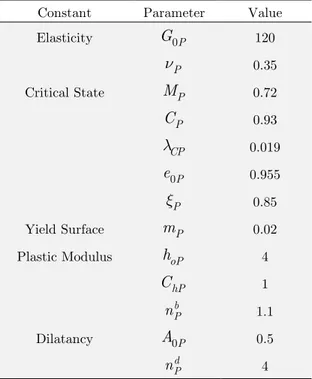
4 DETERMINING MODEL CONSTANTS
Constant Parameter Value
Elasticity G0P 120
P
n 0.35
Critical State MP 0.72
P
C 0.93
CP
l 0.019
0P
e 0.955
P
x 0.85
Yield Surface mP 0.02
Plastic Modulus hoP 4
hP
C 1
b P
n 1.1
Dilatancy A0P 0.5
d P
n 4
Table 2: Values of constants in the plane.
5 RESULTS AND DISCUSSION
In the present research, the fabric effect has been modelled using the multilaminate model framework. Based on microscopic observations, the sandy soil particles should demonstrate contraction behaviour during inverse load, when they are placed in dilatancy condition. To modify their model, Manzari and Dafalias (1997) used the fabric effect in the equations of factor D, using constants CZ and
max
Figure 4: The results of cyclic loading (Dafalias-Manzari method) without
the effect of fabric constants at e0 = 0.808 and p0 = 294kPa.
Figure 5: The results of cyclic loading (Dafalias-Manzari method) with effect
of fabric constants at e0 = 0.808 and p0 = 294kPa.
Figure 6: The results of cyclic loading via multilaminate method and removal of fabric constants.
-1 -0.5 0 0.5 1 1.5 2 2.5 3
-200 -100 0 100 200
Axial strain(%)
q(
kP
a)
0 50 100 150 200 250 300
-200 -100 0 100 200
p(kPa)
q(
kP
a)
(b) (a)
-1 -0.5 0 0.5 1 1.5 2 2.5 3 3.5 4
-200 -100 0 100 200
Axial strain(%)
q(
kP
a)
0 50 100 150 200 250 300
-200 -100 0 100 200
p(kPa)
q(
kP
a)
(a)
(b)
-1 -0.5 0 0.5 1 1.5 2 2.5 3
-200 -100 0 100 200
Axial strain(%)
q(
kPa
)
0 50 100 150 200 250 300
-200 -100 0 100 200
p(kPa)
q(
kPa
)
p0=294kPa,e0=0.808***Multilaminate
p0=294kPa,e0=0.808***Multilaminate
(a)
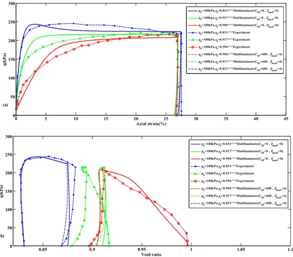
To study more about the effect of the removal of constants related to the fabric in the multilami-nate framework in different loading conditions, void ratio, and confining pressure, the numerical results of constantsCZP = 600andZmaxP = 4 (resulting from calibration) were compared to their removal conditions or zero constants (Figures 7-12). To verify the numerical simulation of the model, the results were compared to the results obtained from the triaxial standard tests of Verdugo and Ishihara (1996). According to the wide changes of confining pressure on the samples from 100kPa to 3000kPa and void ratio from 0.735 to 0.907, results were evaluated in various void and confining pressure conditions during loading and unloading.
The drained condition, with p0 = 100kPa and different
e
0 for the multilaminate model, has been compared to the experimental results in Figure 7. This comparison was done with the above condition for p0 = 500kPa, as shown in Figure 8. The results show the prediction ability of the model in different conditions, such as softening of dense sand particles.Figure 7: Comparison of experimental results and multilaminate modelling for monotonic loading and
unloading in drained standard triaxial test at p0 = 100kPa with and without fabric constants.
0 5 10 15 20 25 30 35 40 45
0 50 100 150 200 250 300
Axial strain(%)
q(
kPa
)
p0=100kPa,e0=0.831***Multilaminate(CZP=0 , ZmaxP=0) p0=100kpa,e0=0.917***Multilaminate(CZP=0 , ZmaxP=0)
p0=100kPa,e0=0.996***Multilaminate(CZP=0 , ZmaxP=0) p0=100kPa,e0=0.831***Experiment
p0=100kPa,e0=0.917***Experiment p0=100kPa,e0=0.996***Experiment
p0=100kPa,e0=0.996***Multilaminate(CZP=600 , ZmaxP=4)
p0=100kPa,e0=0.917***Multilaminate(CZP=600 , ZmaxP=4)
p0=100kPa,e0=0.831***Multilaminate(CZP=600 , ZmaxP=4)
(a)
0.85 0.9 0.95 1 1.05 1.1
0 50 100 150 200 250 300
Void ratio
q(
kP
a)
p0=100kPa,e0=0.831***Multilaminate(CZP=0 , ZmaxP=0) p0=100kPa,e0=0.917***Multilaminate(CZP=0 , ZmaxP=0)
p0=100kPa,e0=0.996***Multilaminate(CZP=0 , ZmaxP=0)
p0=100kPa,e0=0.831***Experiment
p0=100kPa,e0=0.917***Experiment p0=100kPa,e0=0.996***Experiment
p0=100kPa,e0=0.996***Multilaminate(CZP=600 , ZmaxP=4)
p0=100kPa,e0=0.917***Multilaminate(CZP=600 , ZmaxP=4)
p0=100kPa,e0=0.831***Multilaminate(CZP=600 , ZmaxP=4)
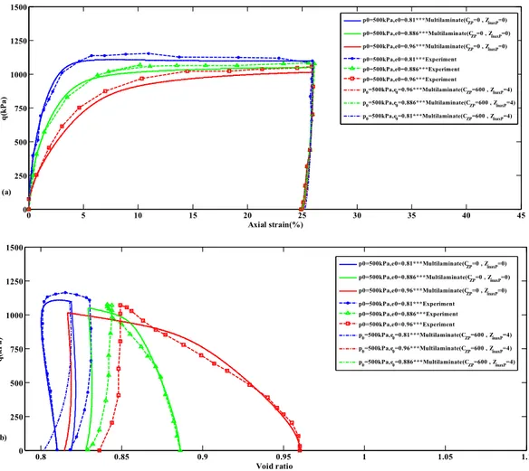
Figure 8: Comparison of experimental results and multilaminate modelling for monotonic loading and
unloading in drained standard triaxial test at p0 = 500kPa with and without fabric constants.
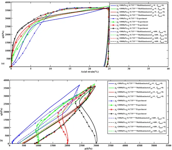
Figure 9 indicate the results for undrained condition, with e0 = 0.735in different confining pres-sures. An important point in the figures is that the steeper gradient of curve p-q is for low confining pressures (p0 = 100kPa ), which matches with the theoretical discussions suggesting the increase in soil angle of internal friction at low pressures and its reduction at high confining pressures.
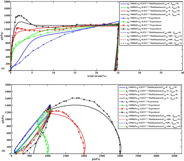
In Figure 10, calibration of the results of the plane constants was done with this void ratio (e0 = 0.833); thus, it is seen to be more in agreement with the experimental results.
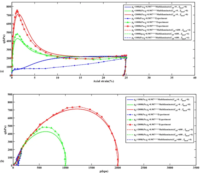
The ability of this model to predict liquefaction appropriately in loose sandy soil with void ratio
0 0.907
e = is shown in Figure 11.
Finally, Figure 12 shows the ability of the model in cyclic loading. Among the remarkable features of the model is the prediction of inverse loading in planes and its effect on the point. The reason for different results in cyclic condition is that cyclic test was done 20 years ago, compared to monotonic tests. This issue can be related by testing method and instrumentation (Dafalias and Manzari, 2004).
0 5 10 15 20 25 30 35 40 45
0 250 500 750 1000 1250 1500
Axial strain(%)
q(
kPa
)
p0=500kPa,e0=0.81***Multilaminate(CZP=0 , ZmaxP=0) p0=500kPa,e0=0.886***Multilaminate(CZP=0 , ZmaxP=0)
p0=500kPa,e0=0.96***Multilaminate(CZP=0 , ZmaxP=0) p0=500kPa,e0=0.81***Experiment
p0=500kPa,e0=0.886***Experiment p0=500kPa,e0=0.96***Experiment
p0=500kPa,e0=0.96***Multilaminate(CZP=600 , ZmaxP=4) p0=500kPa,e0=0.886***Multilaminate(CZP=600 , ZmaxP=4)
p0=500kPa,e0=0.81***Multilaminate(CZP=600 , ZmaxP=4)
(a)
0.8 0.85 0.9 0.95 1 1.05 1.1
0 250 500 750 1000 1250 1500
Void ratio
q(
kP
a)
p0=500kPa,e0=0.81***Multilaminate(CZP=0 , ZmaxP=0)
p0=500kPa,e0=0.886***Multilaminate(CZP=0 , ZmaxP=0)
p0=500kPa,e0=0.96***Multilaminate(CZP=0 , ZmaxP=0) p0=500kPa,e0=0.81***Experiment
p0=500kPa,e0=0.886***Experiment p0=500kPa,e0=0.96***Experiment
p0=500kPa,e0=0.81***Multilaminate(CZP=600 , ZmaxP=4)
p0=500kPa,e0=0.96***Multilaminate(CZP=600 , ZmaxP=4) p0=500kPa,e0=0.886***Multilaminate(CZP=600 , ZmaxP=4)
Figure 9: Comparison of experimental results and multilaminate modelling for monotonic loading and
unloading in the undrained standard triaxial test at e0 = 0.735 with and without fabric constants.
As seen in Figures 7–12, there is not much difference after the removal of parameters related to the fabric effect using the multilaminate method. This can be due to fundamental changes in the calculational principles of the multilaminate method and material behavioural features in the point, resulting from 17 planes instead of three planes. The closeness between the results of the multilami-nate model and the experimental results proves the model capability.
The induced anisotropy effect on post-liquefaction sand particles in 17 directions was studied using related figures (13-16) in the standard triaxial test in monotonic and cyclic conditions. Com-pression and extension were assumed positive and negative respectively in all the modelling. To this end, a sand particle with p0 = 1000kPa and e0 = 0.907 in monotonic and undrained loading and unloading conditions was used for the modelling.
Figure 13 shows the stress path on 17 planes. As seen in Planes 9, 10, 11, 12, and 13, no shear stress is present; there is only pressure. Therefore, such planes are inactive shear and there is no shear strain in these planes (Figure 14). Therefore, these planes have no contribution in the post-liquefaction
0 5 10 15 20 25 30 35 40
0 500 1000 1500 2000 2500 3000 3500 4000
Axial strain(%)
q(
kP
a)
p0=100kPa,e0=0.735***Multilaminate(CZP=0 , ZmaxP=0)
p0=1000kPa,e0=0.735***Multilaminate(CZP=0 , ZmaxP=0) p0=2000kPa,e0=0.735***Multilaminate(CZP=0 , ZmaxP=0) p0=3000kPa,e0=0.735***Multilaminate(CZP=0 , ZmaxP=0)
p0=100kPa,e0=0.735***Experiment p0=1000kPa,e0=0.735***Experiment
p0=2000kPa,e0=0.735***Experiment
p0=3000kPa,e0=0.735***Experiment
p0=100kPa,e0=0.735***Multilaminate(CZP=600 , ZmaxP=4)
p0=1000kPa,e0=0.735***Multilaminate(CZP=600 , ZmaxP=4) p0=2000kPa,e0=0.735***Multilaminate(CZP=600 , ZmaxP=4) p0=3000kPa,e0=0.735***Multilaminate(CZP=600 , ZmaxP=4)
(a)
0 500 1000 1500 2000 2500 3000 3500 4000 4500 5000 5500
0 500 1000 1500 2000 2500 3000 3500 4000
p(kPa)
q(
kP
a)
p0=100kPa,e0=0.735***Multilaminate(CZP=0 , ZmaxP=0)
p0=1000kPa,e0=0.735***Multilaminate(CZP=0 , ZmaxP=0)
p0=2000kPa,e0=0.735***Multilaminate(CZP=0 , ZmaxP=0)
p0=3000kPa,e0=0.735***Multilaminate(CZP=0 , ZmaxP=0) p0=3000kPa,e0=0.735***Experiment
p0=1000kPa,e0=0.735***Experiment
p0=2000kPa,e0=0.735***Experiment p0=3000kPa,e0=0.735***Experiment
p0=100kPa,e0=0.735***Multilaminate(CZP=600 , ZmaxP=4) p0=3000kPa,e0=0.735***Multilaminate(CZP=600 , ZmaxP=4) p0=2000kPa,e0=0.735***Multilaminate(CZP=600 , ZmaxP=4) p0=1000kPa,e0=0.735***Multilaminate(CZP=600 , ZmaxP=4)
lateral spreading. Planes 5, 6, 7, and 8, Planes 1, 2, 3, and 4, and Planes 14, 15, 16, and 17 all follow a stress path to reach failure and liquefaction. This can be studied in Figure 14, where Planes 3 and 4 experience more strain compared to Planes 1 and 2 due to the effect of the similar stress path. The resultant strain determines the movement of soil particles and displacement created in the liquefaction soil in different directions after liquefaction.
Figure 10: Comparison of experimental results and multilaminate modelling for monotonic loading and
unloading in the undrained standard triaxial test at e0 = 0.833 with and without fabric constants.
Eventually, Figures 15 and 16 evaluated the soil behaviour in 17 planes in undrained and cyclic condition under the loading effect of the triaxial standard test with p0 = 294kPa and e0 = 0.808. Figure 15 shows the stress path in the planes. As observed, the value of cyclic shear stress is maximum in Planes 5 and 6 and minimum in Planes 14, 15, 16, and 17. The stress path on each
0 5 10 15 20 25 30 35 40
0 200 400 600 800 1000 1200 1400 1600 1800 2000
Axial strain(%)
q(
kPa
)
p0=100kPa,e0=0.833***Multilaminate(CZP=0 , ZmaxP=0) p0=1000kPa,e0=0.833***Multilaminate(CZP=0 , ZmaxP=0)
p0=2000kPa,e0=0.833***Multilaminate(CZP=0 , ZmaxP=0) p0=3000kPa,e0=0.833***Multilaminate(CZP=0 , ZmaxP=0) p0=100kPa,e0=0.833***Experiment
p0=1000kPa,e0=0.833***Experiment p0=2000kPa,e0=0.833***Experiment p0=3000kPa,e0=0.833***Experiment
p0=100kPa,e0=0.833***Multilaminate(CZP=600 , ZmaxP=4) p0=1000kPa,e0=0.833***Multilaminate(CZP=600 , ZmaxP=4) p0=2000kPa,e0=0.833***Multilaminate(CZP=600 , ZmaxP=4) p0=3000kPa,e0=0.833***Multilaminate(CZP=600 , ZmaxP=4)
(a)
0 500 1000 1500 2000 2500 3000 3500 4000 4500
0 200 400 600 800 1000 1200 1400 1600 1800 2000
p(kPa)
q(
kP
a)
p0=100kPa,e0=0.833***Multilaminate(CZP=0 , ZmaxP=0) p0=1000kPa,e0=0.833***Multilaminate(CZP=0 , ZmaxP=0) p0=2000kPa,e0=0.833***Multilaminate(CZP=0 , ZmaxP=0) p0=3000kPa,e0=0.833***Multilaminate(CZP=0 , ZmaxP=0) p0=100kPa,e0=0.833***Experiment
p0=1000kPa,e0=0.833***Experiment p0=2000kPa,e0=0.833***Experiment p0=3000kPa,e0=0.833***Experiment
p0=3000kPa,e0=0.833***Multilaminate(CZP=600 , ZmaxP=4) p0=2000kPa,e0=0.833***Multilaminate(CZP=600 , ZmaxP=4) p0=100kPa,e0=0.833***Multilaminate(CZP=600 , ZmaxP=4) p0=1000kPa,e0=0.833***Multilaminate(CZP=600 , ZmaxP=4)
plane follows a different pattern to reach liquefaction. It is noteworthy that Planes 7, 8, 9, 10, 11, 12, and 13 are inactive in cyclic conditions in the triaxial standard test, and no shear stress is produced.
Figure 16 indicates shear strain versus shear stress in 17 planes. It should be noted that more shear strain is produced in some planes, such as Planes 5 and 6, while Planes 16 and 17 experience less strain. Therefore, the direction of the post-liquefaction strain in cyclic condition is determined for planes that have more contribution to strain production.
Figure 11: Comparison of experimental results and multilaminate modelling for monotonic loading and
unloading in the undrained standard triaxial test at e0 = 0.907 with and without fabric constants.
0 5 10 15 20 25 30 35 40
0 100 200 300 400 500 600 700 800
Axial strain(%)
q(
kP
a)
p0=100kPa,e0=0.907***Multilaminate(CZP=0 , ZmaxP=0)
p0=1000kPa,e0=0.907***Multilaminate(CZP=0 , ZmaxP=0)
p0=2000kPa,e0=0.907***Multilaminate(CZP=0 , ZmaxP=0) p0=100kPa,e0=0.907***Experiment
p0=1000kPa,e0=0.907***Experiment
p0=2000kPa,e0=0.907***Experiment
p0=2000kPa,e0=0.907***Multilaminate(CZP=600 , ZmaxP=4)
p0=1000kp,e0=0.907***Multilaminate(CZP=600 , ZmaxP=4)
p0=100kPa,e0=0.907***Multilaminate(CZP=600 , ZmaxP=4)
(a)
0 500 1000 1500 2000 2500 3000 3500
0 100 200 300 400 500 600 700 800 900
p(kpa)
q(
kPa
)
p0=100kPa,e0=0.907***Multilaminate(CZP=0 , ZmaxP=0)
p0=1000kPa,e0=0.907***Multilaminate(CZP=0 , ZmaxP=0)
p0=2000kPa,e0=0.907***Multilaminate(CZP=0 , ZmaxP=0)
p0=100kPa,e0=0.907***Experiment
p0=1000kPa,e0=0.907***Experiment
p0=2000kPa,e0=0.907***Experiment
p0=2000kPa,e0=0.907***Multilaminate(CZP=600 , ZmaxP=4) p0=1000kPa,e0=0.907***Multilaminate(CZP=600 , ZmaxP=4)
p0=100kPa,e0=0.907***Multilaminate(CZP=600 , ZmaxP=4)
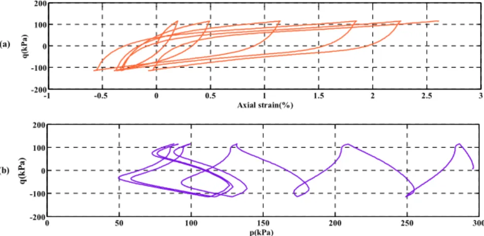
Figure 12: The comparison of experimental (data from Dafalias and Manzari (2004)) results (a,b) and multilaminate modelling for cyclic loading standard triaxial test
at e0 = 0.808 and p0 = 294kPa, with and without fabric constants(c,d).
Figure 13: The shear stress versus normal stress on 17 planes in monotonic
undrained condition, with p0 = 1000kPa and e0 = 0.907.
-0.05 -0.04 -0.03 -0.02 -0.01 0 0.01 -100
-50 0 50 100
Axial strain(in decimal)
q/
2(
kP
a)
0 50 100 150 200 250 300
-100 -50 0 50 100
P(kPa)
q/
2(
kP
a)
p0=294kPa,e0=0.808***Multilaminate(CZP=0 , ZmaxP=0) p0=294kPa,e0=0.808***Multilaminate(CZP=600 , ZmaxP=4) p0=294kPa,e0=0.808***Multilaminate(CZP=0 , ZmaxP=0)
p0=294kPa,e0=0.808***Multilaminate(CZP=600 , ZmaxP=4)
(c) (d)
0 200 400 600 800 1000 1200
0 50 100 150 200 250
Normal stress(kPa)
Sh
ea
r
st
res
s(
kP
a)
Plane1 Plane2 Plane3 Plane4 Plane5 Plane6 Plane7 Plane8 Plane9 Plane10 Plane11 Plane12 Plane13 Plane14 Plane15 Plane16 Plane17 Planes 1,2,3,4
Planes 14,15,16,17
Planes 9,10,11,12,13
Figures 13-16 show that the status of planes, their strain history, and the values of shear strength and strain produced in them in different loading conditions confirm the ability of the model in pre-dicting the induced anisotropy and post-liquefaction occurrences.
Figure 14: The shear stress versus shear strain on 17 planes in monotonic
undrained condition, with p0 = 1000kPa and e0 = 0.907.
Figure 15: The shear stress versus normal stress on 17 planes in cyclic
undrained condition, with p0 = 294kPa and e0 = 0.808.
0 0.2 0.4 0.6 0.8 1 1.2 1.4 1.6
0 50 100 150 200 250
Shear strain
Sh
ea
r
st
res
s(
kP
a)
Plane1 Plane2 Plane3 Plane4 Plane5 Plane6 Plane7 Plane8 Plane9 Plane10 Plane11 Plane12 Plane13 Plane14 Plane15 Plane16 Plane17 Planes 1,2
Planes 14,15
Planes 5,7,8
Planes 16,17
Plane 6 Planes 3,4
0 50 100 150 200 250 300 350 400
-60 -40 -20 0 20 40 60
Normal stress(kPa)
Sh
ea
r
st
res
s(
kP
a)
Plane1 Plane2 Plane3 Plane4 Plane5 Plane6 plane7 plane8 plane9 plane10 plane11 plane12 plane13 plane14 plane15 plane16 plane17
Planes 1,2 Planes 14,15
Plane 6
Planes 3,4
Planes 16,17
Figure 16: The shear stress versus shear strain on 17 planes in cyclic
undrained condition, with p0 = 294kPa and e0 = 0.808.
6 CONCLUSION
In the present research, in addition to the study effect of constant reductions in an advanced consti-tutive model in the multilaminate framework, the effect of induced anisotropy in pre- and post-liquefaction sandy soil is evaluated. In this framework, the constitutive model in the planes is simpli-fied and the costs of experiments and calculations are reduced in practice. In the multilaminate method, the constitutive model was used in 17 planes with different directions instead of in three planes. This can increase the accuracy of the calculations. If the conditions are provided to define different constants in various planes via the experimental results based on soil properties under the initial condition, or even if different constitutive equations are used for different planes, the effect of initial anisotropic condition on soil behaviour can be properly evaluated after loading with this method.
The ability of the multilaminate model in predicting sand particle behaviour in different condi-tions and the start of liquefaction for different values of pressure and void ratio, boundary condition of drained and undrained, cyclic, and monotonic loadings was compared to the experimental results of triaxial standard test and good results were obtained.
Stress-strain behaviour was studied in 17 planes to investigate the model performance in induced anisotropy, liquefaction occurrence, and post-liquefaction conditions. Different values of stress and strain in planes show that the induced anisotropy is affected by loading condition and plane arrange-ment; it proves the ability of the new model for the estimation of such anisotropy. This is especially important in liquefaction soil under different topographic condition, in situ stress and strain, to predict their behaviour and displacements occurring after liquefaction.
Multilaminate model framework provides rotation of the principal axis of stress and lack of co-axiality of principal stress and strain and involves the effects of partial changes in boundary condition, as it protects directional effects in material behaviour. Such subjects and other capabilities of the model can be evaluated in further research works.
-0.01 -0.005 0 0.005 0.01 0.015 0.02 0.025 0.03
-60 -40 -20 0 20 40 60
Shear strain
Sh
ea
r
st
res
s(
kP
a)
Plane1 Plane2 Plane3 Plane4 Plane5 Plane6 Plane7 Plane8 Plane9 Plane10 Plane11 Plane12 Plane13 Plane14 Plane15 Plane16 Plane17
Planes 3,4
Planes 1,2
Planes 14,15
Plane 6 Planes 16,17
References
Basari E., Ozden G. (2013). Post-liquefaction volume change in micaceous sandy soils of Old Gediz River Delta , Acta Geotechnica Slovenica 1:33-40.
Bazant Z. P., Xiang Y. , Adley M. D., Prat P. C., Akers S. A.(1996). Microplane model for concrete: II: data delocal-ization and verification, Journal of Engineering Mechanics;122(3):255-262.
Caner F. C., Bazant Z. P.(2000). Microplane model M4 for concrete. II: Algorithm and calibration, Journal of Engi-neering Mechanics 126(9):954-961.
Chang C. S., Hicher P. Y.(2005). An elasto-plastic model for granular materials with microstructural consideration,
International Journal of Solids and Structures 42:4258–4277.
Dafalias Y. F.(1986). Bounding surface plasticity. I: Mathematical foundation and hypoplasticity, Journal of Engineer-ing Mechanics 112(9):966-987.
Dafalias Y. F., Manzari M. T.(2004). Simple Plasticity Sand Model Accounting for Fabric Change Effects, Journal of Engineering Mechanics 130:622-634.
Dafalias Y. F., Papadimitriou A. G., Li X. S.(2004). Sand Plasticity Model Accounting for Inherent Fabric Anisotropy, Journal of Engineering Mechanics 130(11):1319-1333.
Elgmal A. , Yang Z. Parra E. (2002). Computational modeling of cyclic mobility and post-liquefaction site response, Soil Dynamics and Earthquake Engineering 22:259-271.
Gao Z., Zhao J., Li X. S., Dafalias Y F.(2014). A critical state sand plasticity model accounting for fabric evolution, International Journal for Numerical and Analytical Methods in Geomechanics 38(4):370-390.
Ghadrdan M., Sadrnejad S. A.(2015). Numerical evaluation of geomaterials behavior upon multiplane damage Model, Computers and Geotechnics 68:1-7.
Guo N., Zhao J.(2013). The signature of shear-induced anisotropy in granular media, Computers and Geotechnics 47:1-15.
Guo P.(2014). Coupled effects of capillary suction and fabric on the strength of moist granular materials, Acta
Me-chanica 225:2261-2275.
Hareb H.,Doanh T.(2012). Probing into the strain induced anisotropy of Hostun RF loose sand, Granular Matter 14:589–605.
Hicher P. Y., Chang C. S.(2007). A microstructural elastoplastic model for unsaturated granular materials,
Interna-tional Journal of Solids and Structures 44:2304-2323.
Ishikawa A.,Zhou Y. G., Shamoto Y.,Mano H.,Chen Y. M.,Ling D. S. (2015). Observation of post- liquefaction pro-gressive failure of shallow foundation in centrifuge model tests , Soils and Foundations 55(6):1501–1511.
Khalili Y., Mahboubi A.(2014). Discrete simulation and micromechanical analysis of two-dimensional saturated gran-ular media, Particuology 15:38-150.
Kruyt N. P., Rothenburg L.(2016) A micromechanical study of dilatancy of granular materials, Journal of the
Me-chanics and Physics of Solids 95:411-427.
Kruyt N. P.,Rothenburg L.(2014). On micromechanical characteristics of the critical state of two-dimensional granular
materials, Acta Mechanica 225:2301-2318.
Lashkari A.(2009). A constitutive model for sand liquefaction under rotational shear, Iranian Journal of Science and Technology 33:31-48.
Li X. S.(2002). A sand model with state dependent dilatancy, Geotechnique 52(3):173-186.
Li X., Yu H. S.(2014). Fabric, force and strength anisotropies in granular materials: a micromechanical insight, Acta
Mechanica 225:2345-2362.
Louis L., Baud P., Wong T. F.(2009). Microstructural Inhomogeneity and Mechanical Anisotropy Associated with
Bedding in Rothbach Sandstone, pure and applied geophysics 66:1063–1087.
Manzari M. T., Dafalias Y. F.(1997). A critical state two-surface plasticity model for sands, Geotechnique 47(2):255-272.
Naylor D. J.(1974). Stresses in nearly incompressible materials by finite elements with application to the calculation of excess pore pressures, International Journal for Numerical Methods in Engineering 8(3):443-460.
Sadrnejad S. A. (2007). A general multi-plane model for post-liquefaction of sand, Iranian Journal of Science & Tech-nology, Transaction B, Engineering 31( B1):123-141.
Sadrnejad S. A.( 2011).Soil Plasticity and Modeling(2th ed). Khajeh Nasir Toosi University of Technology(Tehran). Sadrnejad S. A.(2009). Semi-Micro Bounding Surface Model for Anisotropic Sand, Electronic Journal of Geotechnical Engineering 14:1-25.
Sadrnejad S. A., Daryan A. S.,Ziaei M.(2009). A Constitutive Model for Multi-Line Simulation of Granular Material Behavior Using Multi-Plane Pattern, Journal of Computer Science 5(11):822-830.
Sadrnejad S. A., Karimpour H.(2011). Drained and undrained sand behaviour by multilaminate bounding surface model, International Journal of Civil Engineering 9(2):111-125.
Sadrnejad S. A., Labibzadeh M.(2006). A Continuum/Discontinuum Micro Plane Damage Model for Concrete. Inter-national Journal of Civil Engineering 4(4):296-313.
Shamoto Y. , Zhang J. M. , Tokimatsu K. (1998). New charts for predicting large residual post-liquefaction ground
deformation, Soil Dynamics and Earthquake Engineering 17 :427-438.
Taiebat M., Jeremic B., Dafalias Y. F.,Kaynia A. M., Cheng Z.(2010). Propagation of seismic waves through liquefied soils, Soil Dynamics and Earthquake Engineering 30:236-257.
Taiebat M., Dafalias Y. F.(2008). SANISAND: Simple anisotropic sand plasticity model, International Journal for Numerical and Analytical Methods in Geomechanics 32:915-948.
Tam H. K.(1992). Some applications of cam-clay in numerical analysis. Ph.D. Thesis, City University London,England. Tang Tron Tran H., Wong H., Dubujet Ph, Doanh T.(2014). Simulating the effects of induced anisotropy on liquefac-tion potential using a new constitutive model, Internaliquefac-tional Journal for Numerical and Analytical Methods in Geome-chanics 38(10):1013-1035.
Verdugo R. , Ishihara K.(1996). The steady state of sandy soils, Soils and Foundations 36(2):81-91.
Voyiadjis G. Z., Thiagarajan G.,Petrakis E.(1995). Constitutive modelling for granular media using an anisotropic
distortional yield model, Acta Mechanica 110:151-171.
Wang G.,Xie Y.(2014). Modified Bounding Surface Hypoplasticity Model for Sands under Cyclic Loading, Journal of Engineering Mechanics 140:91-101.
Wang R., Zang J. M., Wang G.(2014). A unified plasticity model for large post-liquefaction shear deformation of sand, Computers and Geotechnics 59:54-66.
Wang S. , Luna R., Onyejekwe S. (2015). Postliquefaction behavior of low-plasticity silt at various degrees of recon-solidation , Soil Dynamics and Earthquake Engineering 75:259-264.
Wang Z. L., Dafalias Y. F., Shen C. K.(1990). Bounding surface hypoplasticity model for sand, Journal of Engineering Mechanics 116(5):983-1001.
Yan W. M.(2009). Fabric evolution in a numerical direct shear test, Computers and Geotechnics 36:597–603. Yang Z. X., Li X. S., Yang J.(2008). Quantifying and modeling fabric anisotropy of granular soils, Geotechnique 58(4):237-248.
Ye B., Ye G., Zang F.(2012). Numerical modeling of changes in anisotropy during liquefaction using a generalized constitutive model, Computers and Geotechnics 42:62-72.
Yu H., Zeng X., Li B., Ming H. (2013). Effect fabric anisotropy on liquefaction of sand, Journal of Geotechnical and Geoenvironmental Engineering 139:765-774.
Zhang J. M., Wang G.( 2012). Large post-liquefaction deformation of sand, part I: physical mechanism, constitutive description and numerical algorithm, Acta Geotechnica 7:69-113.