Rev. bras. gest. neg. vol.19 número66

(1)

574

© FECAP

RBGN

574

Review of Business Management

DOI: 10.7819/rbgn.v19i66.2943 Received on

01/28/2016 Approved on 07/24/2017

Responsible editor: Prof. Dr. Eduardo Contani

Evaluation process:

Double Blind Review

Feasibility analysis of the development of an

oil field: a real options approach in a

production sharing agreement

Marcelo Nunes Fonseca

Universidade Federal de Itajubá, IEPG, Itajubá, Brazil

Edson Oliveira Pamplona

Paulo Rotela Junior

Universidade Federal da Paraíba, DEP, João Pessoa, Brazil

Victor Eduardo de Mello Valério

Abstract

Purpose – he aim of this research is to analyze the feasibility of developing a real oil field in Africa under a production sharing agreement, through the application of the real options theory.

Design/methodology/approach – The research was conducted according to the principles of modeling and simulation, based on a structure that consists of three phases, in order to facilitate project feasibility analysis.

Findings – Initially, according to the traditional method, we suggest that the decision-maker does not invest in the development of the ield. However, by incorporating uncertainty into the decision-making process, other results were obtained. Although reduced, we attested that there is a likelihood of feasibility. Next, by using the binomial model to represent the process of oil barrel price difusion, the asset value is calculated considering the lexibility of delaying the development of the ield.

Originality/value – he results show that, if a manager has the right to invest in the future and wait for better oil prices, postponing the development of an oil ield adds value to his assets. he proposed method is a contribution that ofers subsidies to improve decision-making processes to evaluate investments.

(2)

1 Introduction

Evaluating an oil exploration project is a complex and challenging operation. Increasing attention is being given to planning the development of oil and gas ields, considering the discovery of large reserves of these resources over the last decade (Gupta & Grossmann, 2011).

Thus, Helland and Torgersen (2014) warn that assessing investments in oil projects must be done with great care, mainly due to uncertainties in several variables referring to valuation. Uncertainties are deined as deviations from the expected result.

The main sources of uncertainty in decision-making concerning the value of a project are the quantity and quality of a ield’s reserves – an internal variable deined by geological factors – and oil prices – an external variable deined by market factors (Gupta & Grossman, 2014; Helland & Torgersen, 2014; Salomão & Grell, 2001).

According to Schiozer, Ligero and Santos (2004), these uncertainties can inluence the success of oil exploration and production, and, as investments and oil exploration costs have increased rapidly over the past decade, a consistent analytical process that provides an optimal decision is crucial while analyzing investment projects within the oil industry (Helland & Torgersen, 2014).

here are a number of analytical tools that can be used, particularly to evaluate projects involving investments in oil exploration, among which the Discounted Cash Flow (DCF) is a highlight. However, this technique does not take into account the value of managerial lexibility in these types of projects (Helland & Torgersen, 2014).

In this context, the Real Options heory (ROT) is a method capable of incorporating the managerial flexibilities that traditional methods fail to incorporate. According to Fleten, Gunnerud, Hem and Svendsen (2011), valuation through real options has been applied to oil

projects for a long time, since they ofer several attributes that make them suitable for such an evaluation.

As to the methods used to calculate option values, the Black & Scholes model and the binomial tree can be mentioned. In these models, definition requires six variables: the present value of future cash lows, the present value of investments, the risk-free interest rate, the option expiration period, the basic asset’s dividend (or convenience) rate, and the volatility of the basic asset. Among these variables, volatility is highlighted, since, according to Costa Lima and Suslick (2006), this parameter is key and hard to estimate, because there is no historical series of project values.

This scenario of uncertainty has been affecting investments in oil exploration and production in Africa, in which the ield of this study is located. For conidentiality’s sake, only the continent is mentioned; the name of the ield and its country of origin has been kept conidential. According to an Energy Information Administration (2015) publication, only one company was successful in pre-salt exploration in that country. To the aforementioned publication, a combination of disappointing results and geological complexity, aggravated by low oil prices, resulted in reduced investments in pre-salt areas.

Considering these premises, the main objective of this study is to analyze the feasibility of developing an oil ield in Africa, in which a production sharing contract is adopted. In order to attain the objective of this study, a combination of techniques are applied in a real case with the following speciic objectives: (i) to measure the production proile through a three-dimensional (3D) model using Eclipse®_{and Petrel}®_software;

(3)

576

2 Contractual arrangements

As to the ownership of liquid and gaseous hydrocarbons found in that country, the state attributes exclusive rights over these resources to the national concessionaire. In this manner, any oil company (OC) that expects to explore oil in the country should associate with the concessionaire.

Concerning the forms of association, the most frequently used models in that country are:

(i) Production sharing agreement (PSA); and

(ii) Risk service contract (RSC).

2.1 Production sharing agreement (PSA)

he PSA, which emerged in the 1960s in Indonesia, is a very popular method for developing state reserves, particularly in Africa. he characteristics of the PSA are that petroleum resources are the host government’s properties (often represented by the national utility), while the OCs bear all the risks as well as the cost of exploration. In this model, production is divided into an agreed rate between the concessionaire and the OC (or consortium, made up of domestic and/or foreign companies) (Liu, Zhen, Lin, Yanni & Fei, 2012).

hrough the PSA, the host state contributes to the territorial area to be explored, granting the OC (or consortium) the exclusive right to conduct exploration and production activities; however, without entailing any form of lease or transfer of ownership. he OC then explores the area at its own risk and cost, and receives some of the hydrocarbons produced as a compensation for the borne risk. hus, if no hydrocarbons are found or the reserves are not tradable, the contract ends without the OC having any right to recover its costs.

If the activity is successful, the consortium will gain the opportunity to recover the costs incurred and make a proit. In addition, the state and national concessionaire receive a share of the production. In this model, two important

nomenclatures emerge. he irst is Cost Oil, which is the part of the production destined to the consortium, with the purpose of recovering the investments through exploration, development costs, production, administration, and service expenses.

he second is Proit Oil, which is the diference between the total oil produced and the cost recovery oil (Cost Oil). Proit Oil is shared between the concessionaire and the consortium, in accordance with the conditions established in the contract. he tax afects only Proit Oil.

Some characteristics of the production sharing model are described below:

(i) Cost Oil is limited to a maximum percentage of the total amount of oil, generally 50%, and may reach 65% if development and production costs are not recovered within four to ive years after commercial production begins;

(ii) Although Cost Oil is intended for the recovery of investments and total costs incurred, investments in exploration are not taken into account for the eventual increase in the percentage of remuneration; (iii) Development costs are increased

by a factor (uplift) deined in the respective PSA, and amortized at an annual rate of 25%, in the year in which they occur or in the irst year of commercial production, whichever is later;

(iv) he only incident tax is the petroleum income tax (IRP). his tax afects the portion of Proit Oil destined to the consortium, a rate that varies between 30% for domestic companies and 50% for companies of foreign origin.

3 Petroleum exploration and

production

(4)

Grossmann (2014), the life cycle of a typical oil ield project at sea consists of the following ive steps:

(i) Exploration: his activity involves geological and seismic studies, followed by exploratory wells, in order to determine the presence of oil and/or gas;

(ii) Appraisal: This is the drilling of delineation wells to establish the size and quality of the potential field. Preliminary development planning and feasibility studies are also undertaken;

(iii) Development: Following a positive phase of evaluation, this phase aims to select the most appropriate development plan among several alternatives. This stage involves investment and capital intensive investment decisions that include facilities, drilling, and underwater structures, among others;

(iv) Production: After facilities are built and wells drilled, production begins, and gas and/or water can be injected into the ield, in order to increase productivity;

(v) Abandonment: his is the last phase of an oil ield development project and involves dismantling of the facilities.

In case of positive results in the evaluation phase, development is undertaken; this is a set of activities aimed at enabling the commercial production of oil. According to Fleten, Gunnerud, Hem, and Svendsen (2011), and Dixit and Pindyck (1994), the most important decisions in a petroleum exploration and production project refer to the development phase, in which the bulk of the investment takes place.

3.1 Oil price movement

According to Fleten, Gunnerud, Hem, and Svendsen (2011), from the year 2000 in, oil prices have been increasingly volatile, thus

creating uncertainty as to whether projects can deliver suicient returns on investment. hus, the authors state that the price of oil is one of the most important factors in the evaluation of a potential oil ield. Similar to the price of other marketable items, the price of oil is governed by supply and demand.

In 2015, the price drop was alarming. According to a report published by the World Bank (2015), the oil price fell approximately 55% from June 2014 to January 2015, declining from US$115 per barrel to US$47 per barrel, ending a period of four years of stability. he average oil price in 2015 was US$48.67 per barrel, 48% lower than the 2014 average of US$93.17. In January 2016, the price dropped to US$35.97, reaching US$45.60 per barrel in September of the same year.

he changes in oil price are challenging to predict as they luctuate with new information in the market. Considering this, stochastic processes are useful for forecasting, and consequently to indicate the risk of these forecasts through forecast conidence intervals. Considering such complexity, several researches focused on inding better approximations for the behavior of this variable.

Postali and Picchetti (2006) present a discussion on stochastic processes to evaluate investments in the oil and gas sector. he objective of the authors is to present the advantages and disadvantages of the methods of GBM and moving average reversion in the oil price forecast. According to their results, although the average reversal process may be more accurate to represent the evolution of oil prices over a certain period of time, the GBM approximation does not cause signiicant valuation errors. herefore, the results suggest that it is possible to use the GBM as a good method to describe price movement and take advantage of its operational ease.

(5)

578

study to assist in the decision-making on the best continuous-time stochastic models for these risk factors. Tests have shown that the GBM with jumps is the best model to forecast the price of oil, when compared to the other commonly used processes.

In addition, many authors use the GBM method and highlight the importance of this method to model the oil price (Al-Harthy, 2007; Aspen, 2011; Brennan & Schwartz, 1985; Chen Deng, Huang & Quin, 2015; Liu et al., 2012; Meade, 2010; Mostafaei, Sani & Askani, 2013; Paddock, Siegel & Smith 1988). hus, despite several techniques to model the movement of oil prices, considering the research of the main authors in this subject, it can be concluded that the stochastic model of GBM presents robust approximations, as the standard deviations of the results are within the prediction interval and do not generate signiicant evaluation errors (Pindyck, 1999).

3.1.1 Geometric Brownian Motion (GBM)

According to Dixit and Pindyck (1994), the Brownian motion (or Wiener process) is a stochastic process that presents the following three important properties:

(i) This is a Markov process, and therefore the probability distribution for all future values depend only on the present value;

(ii) The process has independent increments. hus, over a period of time, the probability distribution for the variations in the process is not afected by another time interval;

(iii) Changes in the process during any time interval are normally distributed, increasing the variance linearly with time interval.

According to Dixit and Pindyck (1994), a variable P follows a GBM if it follows the stochastic diferential equation below, since P(0) is the known value at t = 0:

1)

where

α: growth rate (drift); σ: volatility (σ > 0);

dz: increment of the Wiener process

(

In the GBM, variable P follows a lognormal distribution, since the percentage rate of variation of the stochastic variable (dP/P) follows a normal distribution with the mean and variance shown below:

2)

Considering x = Ln P and using Itô’s lemma, we obtain:

3)

(6)

4)

5)

Assuming risk neutrality, and thus using the risk-free rate (r) instead of the growth rate (α), we obtain:

6)

hrough mathematical transformations, equation (6) can be written as follows:

7)

In order to determine the variable P(T) at date T, equation (7) indicates that the following four variables need to be deined: initial value P(0), risk free interest rate (r), volatility (σ), and the random number (N (0,1)).

According to Dias (2015), if P follows a GBM, considering the initial value of P (P0), then its future values P(t) have lognormal distributions with the following mean and variance:

8)

9)

Assuming risk neutrality, the growth rate α is replaced by the risk premium penalized (α - π), where π is the risk premium. However, we obtain (α - π) = (r - δ), where r is the risk free rate and δ is the convenience rate.

he convenience rate is related to the possibility of a product shortage, which could unexpectedly interrupt production and is analogous to the dividend rate of a inancial asset; however, in this case, the asset is a commodity (Dias, 2015). The convenience rate can be calculated by the mean of equation (10) (Fleten, Gunnerud, Hem & Svendsen, 2011).

10)

Here, r is the risk-free rate, P(t) the spot price, and F(P, t, T) are the future market prices at a generic instant t for delivery on date T.

In the case of risk-neutral GBM, the mean and variance are calculated as follows:

11)

12)

4 Real options

he decisions referring to oil exploration and production are complex, mainly due to the high number of uncertainties involved (Suslick, Schiozer & Rodriguez, 2009). According to Schiozer, Ligero and Santos (2004), uncertainties are those that can influence the success of oil exploration and production. Although signiicantly new methodologies for measuring the uncertainties have been found, they do not accurately deine the impact of uncertainties, as this impact varies with time and the amount of information available.

(7)

580

order to not disregard its value as a method to evaluate projects.

According to Dias (2004), the real options method can be considered as an optimization problem under uncertainty, where in most practical cases, the net present value (NPV) should be maximized, subject to:

(i) Relevant options (managerial lexibility);

(ii) Market uncertainties (oil price and equipment fees);

(iii) Technical uncertainties (existence of oil, and quality and quantity available).

As highlighted by Helland and Torgersen (2014), the main types of real options in most investment projects are abandonment, timing, expansion, and temporary suspension.

4.1 Binomial method

Cox, Ross and Rubinstein (1979) propose a simple model of pricing discrete time options, and it is possible to obtain the same results from the Black and Scholes (1973) model using only elementary mathematics. In order to facilitate the development of the model, it is assumed that an asset can take the following two values in the future:

• Su: S multiplied by the upward factor “u” (up);

• Sd: S multiplied by the backward factor “d” (down).

he values of these multiplying factors, represented by “u” and “d”, respectively, are based on the volatility (σ) of the object asset and the expiration time (Δt), as presented in equations (13) and (14), respectively:

13)

14)

he probability of reaching each node is deined by the letter “p,” which represents the neutral risk probability or equivalent martingale

measure. For Copeland and Antikarov (2001), the risk-neutral probability is only a facilitated method of adjusting the cash lows in order to discount them at a risk-free rate. hus, the neutral probability to upside risk (p_u) and descending risk (p_d) when dividends are obtained, are presented

in equations (15) and (16), respectively.

15)

16)

where:

r_c:risk-free rate in continuous time;

δ_c: dividend rate in continuous time.

When the basic asset is the price of a commodity, is the convenience rate in continuous time.

he process is simple. After generating a binomial tree for multiple periods of the basic asset, calculation of the values of the option using this method is similar to the process of resolution of decision trees visually. In addition, it is a process of retroinduction optimization (backwards). he value of the option is calculated as follows:

17)

At the expiration date (t = T), the value of the option is:

18)

5 Research method

(8)

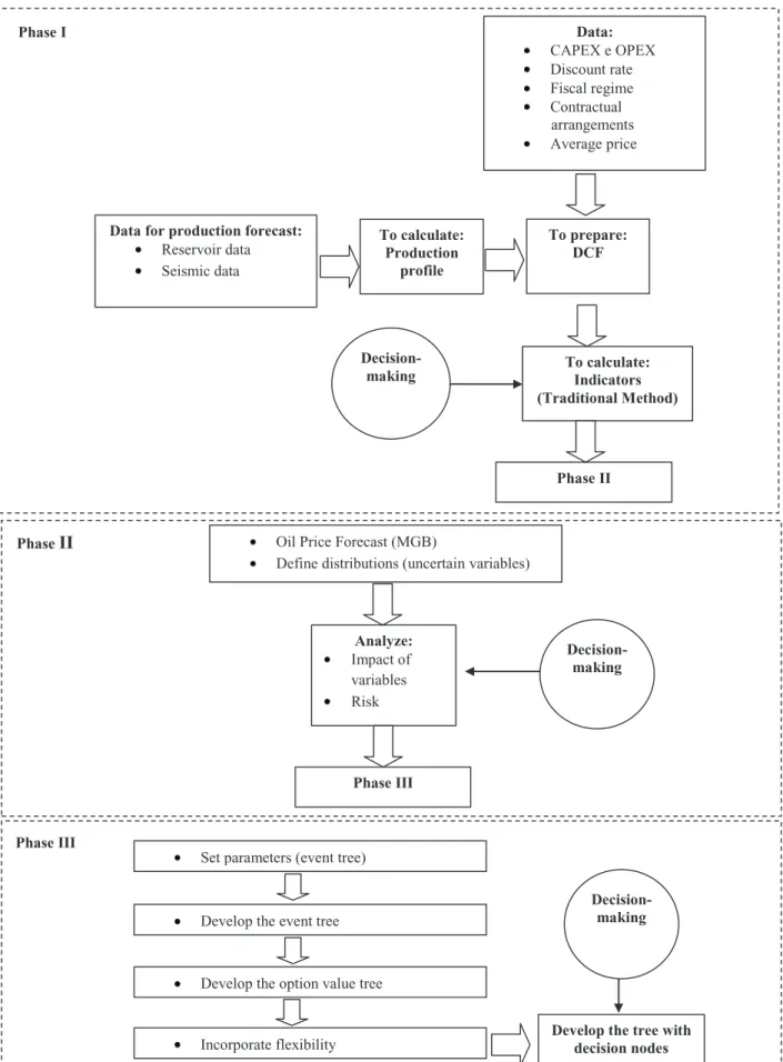
In order to develop systematization for solving the problem of modeling and simulation, a structure was elaborated to support the analysis of the project, under the perspective of the traditional method of analysis of investments, risk, and real options. his structure is outlined in Figure 1.

First of all, geological data, such as luid and rock properties, ield characteristics, and ield seismic data were selected, in order to calculate the ield production proile. he following project data were then collected: planned schedule for CAPEX, schedule of expected values for OPEX, government participations, contract properties, and discount rate. In order to analyze the feasibility of the development of the ield, the cash lows of the production period were obtained. hrough the traditional method of investment analysis, such as NPV and IRR indicators, the feasibility of the ield was analyzed.

The second phase (phase II) started with the forecast of oil prices, using the GBM. Uncertainties referring to the variables CAPEX, OPEX, and production proile were inserted into

the model, in order to investigate their impact on the result obtained in the irst phase. he variables that impact the most were selected, and inally, the risk analysis was performed. At this stage, decisions can be made within a probabilistic scenario.

he irst stage of the last phase (phase III) refers to the choice of a real options model that can translate the efect of the variables that impact the most, selected in the previous phase. Next, the parameters required to create the event tree are calculated. he next step is to incorporate flexibility into the project and calculate the value of the option. he lexibility considered in the present study is postponing the necessary investments in the development of the oil ield under evaluation.

(9)

582 _–

Phase I Data:

CAPEX e OPEX Discount rate Fiscal regime Contractual arrangements Average price

Data for production forecast: Reservoir data Seismic data

To calculate: Production

profile

To prepare: DCF

To calculate: Indicators (Traditional Method)

Decision-making

Phase II

Phase III

Set parameters (event tree)

Develop the event tree

Develop the option value tree

Incorporate flexibility Develop the tree with _{decision nodes}

Decision-making Phase II Oil Price Forecast (MGB)

Define distributions (uncertain variables)

Analyze: Impact of variables Risk

Phase III

Decision-making

(10)

6 Discussion of results

6.1 Phase I - Traditional project analysis

As mentioned earlier, the national concessionaire holds the rights to hydrocarbons and its form of association with the consortium is governed by the PSA. he consortium is made up of two companies, one foreign and one national, in which the rightful percentage is 40% and 60%, respectively.

At the irst moment, in which the objective is to analyze the feasibility of the project through a deterministic model, it is assumed that the average price of a barrel of oil during the production period is equal to the initial price, being P(0) = US$59.80, which is the value referring to the price of a barrel of oil in June 2015.

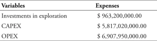
he total expenses of the studied ield are shown in Table 1.

Table 1

E&P Expenses

Variables Expenses

Investments in exploration $ 963,200,000.00

CAPEX $ 5,817,020,000.00

OPEX $ 6,907,950,000.00

Petrel®_{and Eclipse}®_{software were used to}

forecast oil production. hese forecasts represent three possibilities for ield recoveries. he “base case” forecast recovers 280 million barrels from ten production wells, three gas injectors, and three water injectors. he “optimistic case” recovers 460 million barrels from 14 production wells, four gas injectors, and three water injectors. he “pessimistic case” recovers 150 million barrels through six production wells, three gas injectors, and two water injectors. Daily production forecast in thousands of barrels per day (kBOPD) is presented in Figure 2.

Figure 2. Field production proile

Considering the deterministic model, the “base case” will be used. In the PSA, cash lows

(11)

584

Table 2

Consortium cash low model (PSA)

Total revenue (-) OPEX (-) CAPEX

(-) Oil income tax (IRP) (=) Consortium cash low

Since the scope of this study focuses on the feasibility analysis, values referring to each item of the cash low are not speciied.

6.1.1 Traditional method

hrough traditional indicators (NPV and IRR) it is possible to analyze the feasibility of the project. he weighted average cost of capital (WACC) used is 10%, which is the value used by the consortium in the evaluation of development of oil ields in the country which is under analysis.

Table 3 shows NPV and IRR values, from the perspective of the consortium for the PSA.

Table 3

Indexes (traditional evaluation method)

Indexes Value

NPV $ -800,570,000.00

IRR 2.03%

herefore, based on the traditional method of investment analysis, the consortium is advised to not declare the commerciality of the analyzed ield, as the negative NPV indicates infeasibility of the ield development. As mentioned previously, in this manner, the consortium will lose all the investments made in exploration activities, with no possibility of recovery of these values.

6.2 Phase II - Risk analysis

Considering the objective of analyzing whether price is actually an impacting variable in the final result, as well as evaluating the importance of the other input variables of the project (CAPEX, OPEX, and production forecast), a sensitivity analysis was undertaken

considering these variables. he project was then evaluated from a risk perspective.

6.2.1 Sources of uncertainty

Based on the knowledge of company managers, the main sources of uncertainty considered in the project were the following variables:

• Market uncertainty: price of a barrel of oil, CAPEX, and OPEX; and

• Technical uncertainty: production forecast.

Dias (2005), and Pindyck and Rubinfeld (1991) performed the Dickey-Fuller unit root test in respect to the oil price series and did not find evidence that the GBM hypothesis can be rejected. Taking this into consideration, the same test was conducted on the price data set of this study, and according to the aforementioned authors, the p-value were found to be: (a) 0,1810 for a random walk; (B) 0,2772 for a random walk with a displacement e; (C) 0,2377 for a random walk with a deterministic trend shift (GBM).

herefore, the GBM is selected as the technique to be used to predict the price of oil during the production period of the ield. hus, if P follows a GBM considering the initial value of P, then its future values P(t) have lognormal distributions with the mean and variance calculated using equations (8) and (9).

In order to deine the risk-free rate, the yield on the United States of America (the US) Treasury Bond with a 10-year maturity was determined for the period January 2000 to August 2015. he average real annual rate of interest was found to be 2.65%.

(12)

proxy for the current value. herefore, the future price for delivery in one month was used as an approximation of the spot price. Considering the future market price, the WTI oil price data were used for delivery in month 18. hus, the annual convenience rate was 2.92%. his value is consistent with Pickles and Smith (1993), who recommend using δ = r (risk free rate).

According to Dias (2015), if prices follow a GBM, the parameters of volatility (σ) and growth (α) can be estimated with a trivial linear regression. hus, these parameters can be calculated using equations (19) and (20):

19)

20)

hese parameters are usually reported in annual units (% per year), but data is often daily, weekly, or monthly, where N is the number of periods per year of data observation. In the present

case, N will be equal to 12, as monthly data will be analyzed on the price of a barrel of oil.

In order to determine the growth rate (annual) α and the volatility (annual) σ, we used WTI oil (IMF, 2015) in real values (US$ June 2015) delated using the Consumer Price Index as a delator of the US dollar with monthly data from July 2000 to June 2015. he annual growth rate was 7.84% and the volatility was 34.12% per year.

he volatility found in this study was higher than the volatility found by Lund (1999) and Fleten, Gunnerud, Hem, and Svendsen (2011), which can be explained by the high volatility of the oil price in recent years, though it is in close proximity to the volatility (33.07%) found by Dias (2015). he initial price considered is for June 2015, quoted at US$59.80.

Finally, parameters are replaced in equations (8) and (9), and the expected values for the price and diversion of oil during the production period are calculated.

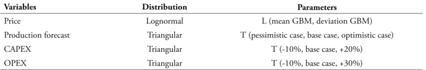
The distributions and parameters that were used are shown in Table 4.

Table 4 Distributions

Variables Distribution Parameters

Price Lognormal L (mean GBM, deviation GBM)

Production forecast Triangular T (pessimistic case, base case, optimistic case)

CAPEX Triangular T (-10%, base case, +20%)

OPEX Triangular T (-10%, base case, +30%)

6.2.2 Sensitivity analysis

he stochastic variables were inserted into the model and using the CrystalBall® _software,

10.000 iterations were simulated.

The sensitivity analysis of the chosen variables shows that price is the variable that has the most impact in the inal result. he other

(13)

586

120 100

80 60

40 20

4000

3000

2000

1000

0

-1000

-2000

-3000

-4000

Preço

V

a

lo

r

P

re

s

e

n

te

L

íq

u

id

o

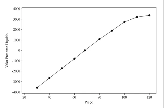
Figure 3. NPV x Price

Table 5 Decision rule

Price Decision

P< US$68.30 Do not invest

P≥ US$68.30 Invest

herefore, from the perspective of the consortium, if managers choose to base their decisions on a deterministic analysis, disregarding the risks and lexibilities of the project, and in a scenario of oil prices above US$68.30, the area under evaluation may be declared commercial.

6.2.3 Project risk

After entering the distribution of the most sensitive variable of the project (price of oil barrel) through Monte Carlo simulation, CrystalBall®

software provides the distribution of the possible NPV results.

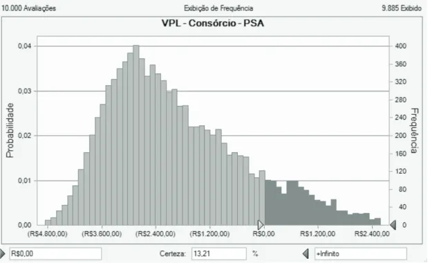
Figure 4 shows that the probability of feasibility, that is, of obtaining an NPV above zero, is equal to 13.21%. However, considering

decision making using the NPV metric, managers would probably not choose to invest in the development of the ield.

hus, we can observe that the negative results presented in both contracts are mainly relected in the price of oil, which has been showing a steep decline in recent years. hus, Helland and Torgersen (2014), Gupta and Grossman (2014), and Fleten, Gunnerud, Hem, and Svendsen (2011) highlight that the fluctuation of oil prices are one of the most important variables in the analysis of investments in oil projects. Also conirming the justiications for the unfavorable scenario of investments in oil in the country where the ield is located, is published by the Energy Information Administration (2015).

(14)

Figure 4. Project risk

6.3 Phase III - he value of lexibility

At this stage, an application of the multiperiod binomial method will be undertaken as the object of this study, in order to capture the value of the lexibility of this project. However, the binomial model will be used to represent the process of price difusion of the barrel of oil, which is the basic asset. Considering the present project,

it is assumed that, from 2015 on, the consortium will have ive years to begin the development of the ield. hus, calculating the value of the option to postpone investments (waiting option) for the development of the oil ield under the perspective of the PSA is preferred.

he parameters for calculating the value of lexibility are presented in Table 6.

Table 6

Parameters of RSC

Parameters Values

Initial price (P0) $59.80

Volatility 34.12%

Convenience fee (per year) 2.92%

Risk free rate (per year) 2.65%

Field life 20

Time interval in the tree (Δt) 1

Tree stages 5

Expiration time (T) 5

Upward factor (u) 1.4066345

Downward factor (d) 0.7109167

Neutral probability to risk (p) 41.11%

(15)

588

6.3.1 Real Options

Having calculated the parameter values, the binomial method for option pricing was developed according to the four phases outlined below, based on the equations described in section 4.1:

(i) Generate the binomial tree of the basic asset V;

(ii) Generate the event tree for the value of the developed ield: the value of the developed asset is a function of the price of the barrel of oil;

(iii) Calculate the value of the asset using the option at the terminal nodes (t = T);

(iv) Calculate backwards, the values of the asset using the option of waiting in the predecessor nodes (t <T) until the initial date (t = 0).

Based on the values of the asset with the hold option, the binomial tree was developed, including lines in which the optimal decision is highlighted (see Table 7), considering that this is a more intuitive tool for the decision maker.

Table 7

Binomial tree (standby option)

2015 2016 2017 2018 2019 2020

Oil barrel prices $59.80 $84.12 $118.32 $166.44 $234.11 $329.31

Decision Standby Standby Standby Invest Invest Invest

Oil barrel prices $42.51 $59.80 $84.12 $118.32 $166.44

Decision Standby Standby Standby Invest Invest

Oil barrel prices $30.22 $42.51 $59.80 $84.12

Decision Standby Standby Standby Invest

Oil barrel prices $21.49 $30.22 $42.51

Decision Standby Standby Quit

Oil barrel prices $15.27 $21.49

Decision Standby Quit

Oil barrel prices $10.86

Decision Quit

The binomial tree shows the possible scenarios of the future price of oil barrel and the indication to the decision maker. For example, if in 2016 the oil price reached US$84.12, in order to maximize the results, the indicated decision is to expect a better time, although the scenario shows that investing in this would provide positive results. It should be noted that the method used considers that the other variables did not change with the passage of time.

It can be observed that the period with the highest number of favorable investment

scenarios is in the year 2020, which is the year of expiration of the option. his occurs due to the high uncertainty captured in the binomial difusion, as the price variance increases with the time horizon such that more extreme price scenarios are present in 2020.

(16)

2020 2019

2018 2017

2016 2015

95

90

85

80

75

70

Período

P

re

ç

o

d

e

G

a

ti

lh

o

Figure 5. Trigger curve

It can be observed from Figure 5 that, at the expiration date of the option (2020), the trigger price is equal to US$68.30, the value from which the project becomes viable.

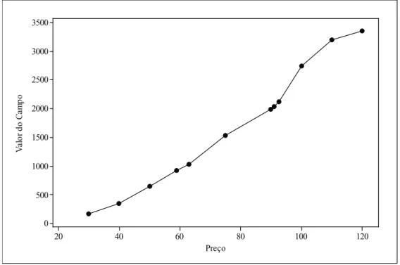
he value of the ield was calculated at $ 924,230,000.00, using the option. Figure 6 shows the value of the ield calculated using the option (in millions of dollars) versus the price of a barrel of oil.

120 100

80 60

40 20

3500

3000

2500

2000

1500

1000

500

0

Preço

V

a

lo

r

d

o

C

a

m

p

o

(17)

590

Therefore, it is possible to verify the importance of the manager, in order to obtain the option to postpone the development of the ield, as the results obtained show that the asset substantially appreciated in this case, when

compared to the result obtained through the traditional method.

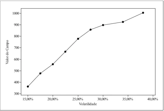
Finally, Figure 7 shows the inluence of volatility on the value of the asset. he value of the oil ield are in millions of dollars.

40,00% 35,00%

30,00% 25,00%

20,00% 15,00%

1000

900

800

700

600

500

400

300

Volatilidade

V

a

lo

r

d

o

C

a

m

p

o

Figure 7. Value of the ield with the option x volatility

As shown in Figure 7, the value of the ield is positively inluenced by the volatility. his result corroborates the analysis that uncertainty of the project has the potential to add value to it, if the manager has the lexibility to delay the development of the ield.

7 Conclusions

This study was based on a real case of economic analysis of investments, with the objective to analyze the feasibility of the development of an oil ield located in Africa, where the PSA was adopted.

he production proile of the oil ield under analysis was created from a 3D model, developed through Petrel®_{and Eclipse}®_software.

he use of this technique provided more precision in the economic feasibility analysis of the project,

as this method is better represented for the ield production potential. In addition, this procedure contributed to literature, as several analyses of oil investments are based on less robust techniques, such as zero-scale models.

However, in order to approximate the investment analysis to the real behavior of the project, the GBM technique was applied to forecast oil prices. Using this approach, a low oil price scenario was found during the production period, and the intensity of this movement signiicantly inluenced the project’s infeasibility when managerial lexibility was disregarded.

(18)

was entered for risk analysis, which resulted in a low likelihood of feasibility of ield development (13.21%), also indicating the decision to not commerciality declare the ield.

Finally, the ROT was used to investigate the value of managerial lexibility in the ield feasibility analysis. From the point of view of real options, it was found that volatility creates value for the project, as the value of the asset increased from US$800,570,000 to US$924,230,000, when managerial lexibility was considered. hus, the indication to maximize the value of the asset is expected by a favorable scenario of oil prices.

The analyses are similar to the reality of low investments in the pre-salt areas of the country in question. his can be explained by comparing the average oil prices for 2015 and 2016, with the trigger prices for the periods, where the option can be exercised, which suggests the manager to wait for better conditions of the price of the barrel, and therefore, to postpone the investments.

However, it should be noted that the project’s volatility was considered to have originated in the price volatility of the oil barrel. his is a contour condition of the present study. hus, as a future research, it is suggested that other variables could be included to obtain less imprecise estimates of the volatility of each project. In addition, another possibility of research is based on the development of the same analysis, but for service contract with risk, and then comparing the results with the present study.

References

Al-Harthy, M. H. (2007). Stochastic oil price models: Comparison and impact. he Engineering Economist,52(3), 269–284.

Aspen, L. (2011). Oil price models and their impact in project economics (Master hesis). University of

Stavanger, Stavanger, Norway.

Armstrong, M., Galli, A., Bailey, W., & Couet, B. (2004). Incorporating technical uncertainty

in real option valuation of oil projects. Journal of Petroleum Science and Engineering, 44 (1-2),

67–82.

Brennan, M. J., & Schwartz, E. S. (1985). Evaluating natural resource investments. Journal of Business, 58(2), 135–157.

Black, F., & Scholes, M. (1973). he pricing of options and corporate liabilities. Journal of Political Economy, 81, 637-659.

Brandão, L., Dyer, J., & Hahn, W. (2005). Using binomial decision trees to solve real-option valuation problems. Decision Analysis, 2(2), p.

69-88.

Chen, R., Deng, T., Huang, S., & Qin, R. (2015). Optimal crude oil procurement under luctuating price in an oil refinery. European Journal of Operational Research, 245(2), 438–445.

Cox, J., Ross, S., & Rubinstein, M. (1979). Option price: A simpliied approach. Journal of Financial Economics, 7(3), 229-264.

Copeland, T. E., & Antikarov, V. (2001).

Opções reais: Um novo paradigma para reinventar a avaliação de investimentos. Rio de Janeiro:

Campus.

Costa Lima, G. A., & Suslick, S. B. (2006). Estimation of volatility of selected oil production projects. Journal of Petroleum Science and Engineering, 54(3-4), 129–139.

Dias, M. A. G. (2004). Valuation of exploration and production assets: An overview of real options models. Journal of Petroleum Science and Engineering, 44(1-2), 93–114.

Dias, M. A. G. (2005). Opções reais híbridas com aplicações em petróleo (Tese Doutorado).

Departamento de Engenharia Industrial, Pontifícia Universidade Católica do Rio de Janeiro, Rio de Janeiro, Brazil.

(19)

592

em petróleo e em outros setores (Vol. 2: Processos

estocásticos e opções reais em tempo contínuo). Rio de Janeiro: Interciência.

Dixit, A. K., & Pindyck, R. S. (1994). Investment under Uncertainty. New Jersey, Princeton:

University Press.

Energy Information Administration – EIA. (2015). Independent Statistics and Analysis.

Retrieved from www.eia.gov.

Fleten, S., Gunnerud, V., Hem, O. D., & Svendsen, A. (2011). Real option valuation of ofshore petroleum ield. Journal of Real Options, 1, 1–17.

Gupta, V., & Grossmann, I. E. (2014). Multistage stochastic programming approach for ofshore oilield infrastructure planning under production sharing agreements and endogenous uncertainties.

Journal of Petroleum Science and Engineering, 124,

180–197.

Gupta, V., & Grossmann, I. E. (2011). Ofshore oilield development planning under uncertainty and iscal considerations. [Working paper, p. 1-43]. Carnegie Mellon University, Pittsburg, EUA. Retrieved from https://pdfs.semanticscholar. org/ceb9/1220e69c2f48184e901136646932a8 2f5dc3.pdf

Helland, J., & Torgersen, M. (2014). he Value of Petroleum Exploration under Uncertainty: A Real Option Approach (Master Tesis). Norwegian

School of Economics, Norway.

Kafel, B., & Abid, F. (2009). A methodology for the choice of the best itting continuous-time stochastic models of crude oil price. he Quarterly Review of Economics and Finance, 49(3),

971–1000.

IMF- International Monetary Fund. (2015). IMF Primary Commodity Prices. Retrieved from www.

imf.org/external/np/res/commod/index.aspx

Liu, M., Zhen, W., Lin, Z., Yanni, P., & Fei, X. (2012). Production Sharing Contract: An analysis based on an oil price stochastic process. Petroleum Science, 9(3), p.408-415.

Lund, M. W. (1999). Real Options in Ofshore Oil Field Development Projects. [Working Paper N-4035, p. 1–27]. Natural Gas Marketing & Supply, Statoil, Stavanger, Norway. Retrieved from http://www.realoptions.org/papers1999/ LUND.PDF

Meade, N. (2010). Oil prices – Brownian motion or mean reversion? A study using a one year ahead density forecast criterion. Energy Economics, 32(6), 1485–1498.

Mostafaei, H., Sani, A. A. R., & Askari, S. (2013). A methodology for the choice of the best itting continuous-time stochastic models of crude oil price: he case of Russia. International Journal of Energy Economics and Policy, 3(2), 137–142.

Paddock, J. L., Siegel, D. R., & Smith, J. L. (1988). Option valuation of claims on real assets: he case of ofshore petroleum leases. Quarterly Journal of Economics, 103, p. 479- 508.

Postali, F. A. S., & Picchetti, P. (2006). Geometric brownian motion and structural breaks in oil prices: A quantitative analysis. Energy Economics, 28(4), 506–522.

Pickles, E., & Smith, J. L. (1993). Petroleum Property Evaluation: A binomial lattice implementation of option pricing theory. Energy Journal, 14(2), 1-26.

Pindyck, R. S., & Rubinfeld, D. L. (1991).

Econometric Models and Economic Forecasts (3rd

ed.). New York: McGraw-Hill, Inc.

Pindyck, R. S. (1999). he Long-Run Evolution of Energy Prices. Energy Journal, 20(2), p. 1-27.

(20)

characterization and low simulation. SPE Latin American and Caribbean Petroleum Engineering Conference. Buenos Aires, Argentina, SPE 69477.

Schiozer, D. J., Ligero, E. L, & Santos, J. A. M. (2004). Risk assessment for reservoir development under uncertainty. he Journal of the Brazilian Society of Mechanical Sciences and Engineering, 26(2), 213-217.

Suslick, S. B.,Schiozer, D., & Rodriguez, M. R. (2009). Uncertainty and risk analysis in petroleum exploration and production. Terrae, 6(1), 30-41.

World Bank (2015). Commodity Markets Outlook.

Retrieved from documents.worldbank.org/ curated/pt/380281468125701579/pdf/938350 WP0Box3805a0commodity0Jan2015.pdf

Supporting agencies:

Fapemig – Fundação de Amparo à Pesquisa de Minas Gerais

CNPq – Conselho Nacional de Desenvolvimento Cientíico e Tecnológico CAPES – Coordenação de Aperfeiçoamento de Pessoal de Nível Superior

About the authors:

1. Marcelo Nunes Fonseca, Master’s Degree in Production Engineering, Universidade Federal de Itajubá. Brazil. E-mail: marcelonunes21@yahoo.com.br

ORCID

0000-0002-3651-8747

2. Edson de Oliveira Pamplona, Doctorate Degree in Management, Fundação Getúlio Vargas. Brazil. E-mail: pamplona@unifei.edu.br

ORCID

0000-0001-6085-0240

3. Paulo Rotela Junior, Doctorate Degree in Production Engineering, Universidade Federal de Itajubá. Brazil. E-mail: paulo.rotela@gmail.com

ORCID

0000-0002-4692-7800

4. Victor Eduardo de Mello Valério, Master’s Degree in Production Engineering, Universidade Federal de Itajubá. Brazil. E-mail: victor.dmv@gmail.com

ORCID

0000-0003-4127-5951

Contribution of each author:

Contribution Marcelo Nunes

Fonseca

Edson de Oliveira Pamplona

Paulo Rotela Junior

Victor Eduardo de Mello

Valério

1. Deinition of research problem √ √

2. Development of hypotheses or research questions

(empirical studies) √ √ √